Recommended resources
The freely available resources this lesson will direct you to.
- This is How Google’s Phone Enhances Your Photoswww.youtube.com
- Marc Levoy - Lectures on Digital Photography - Lecture 10 (20apr16).mp4www.youtube.com
- [PDF] Burst photography for high dynamic range and low-light imaging on ...hdrplusdata.org
- [2102.09000] Mobile Computational Photography: A Tourar5iv.labs.arxiv.org
Hello. In the previous lesson, backside illumination, sensor stacking, miniature optics, and folded light paths each moved a physical constraint without eliminating it. This final lesson asks what happens when the camera instead makes several measurements of the scene and spends computation to combine them.
We will evaluate four results: cleaner images from burst fusion, greater scene dynamic range from computational HDR, shallow-looking depth of field without a large aperture, and finer sampled detail from multi-frame super-resolution. The recurring question is not whether software “replaces” hardware, but which missing measurement it can recover, which assumptions make recovery possible, and what it costs. Allow about 40–45 minutes for the lesson and focused resources.
One camera, several observations
A single exposure must fit competing requirements into one interval. A longer exposure collects more photons but risks subject blur and pixel saturation. A shorter exposure protects motion and highlights but leaves shadows noisy. A small-aperture camera also produces relatively little optical background blur, while its sensor samples fine detail on a finite grid.
Multi-frame imaging gives the camera more observations, not an exemption from these constraints. The observations become useful only if they differ in a helpful way: independent noise realizations can be averaged; different exposure times can cover different brightness ranges; slightly shifted sampling grids can reveal more spatial information. Conversely, scene motion can make two frames describe different scenes rather than repeated measurements of the same one.
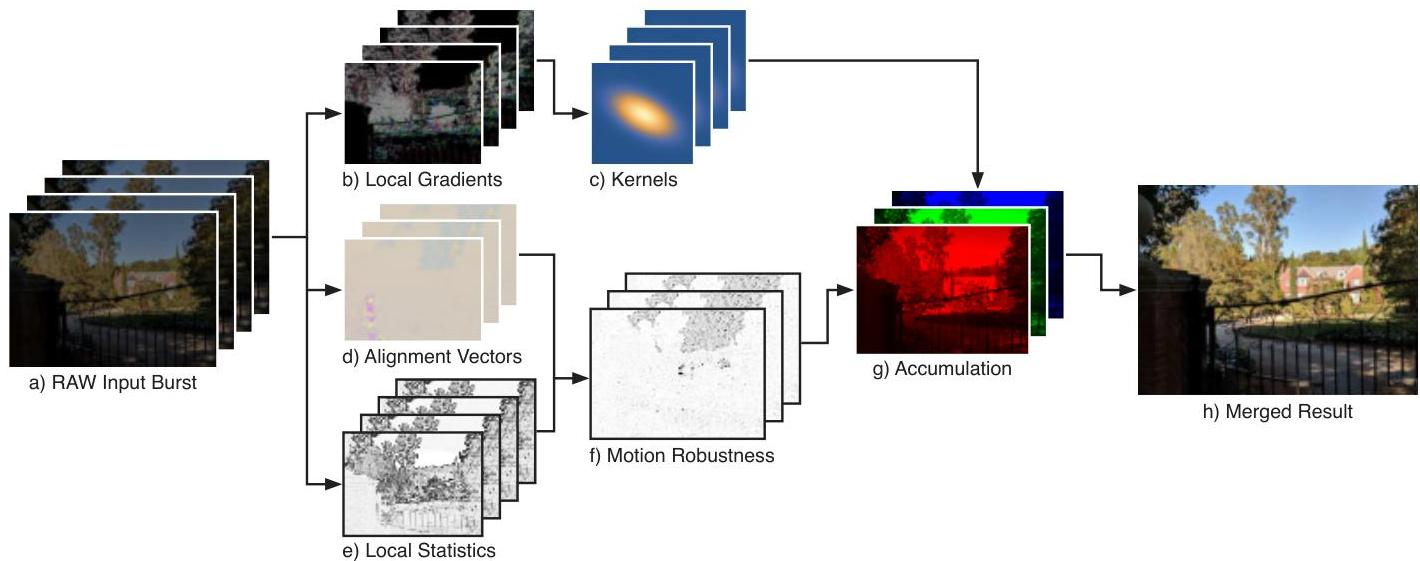
The image below shows the broad idea. Notice that merging raw frames produces an intermediate measurement, not yet the displayed photograph; rendering and tone decisions remain.

For a concrete original system, read the opening and exposure strategy of Hasinoff and colleagues’ Burst Photography for High Dynamic Range and Low-Light Imaging on Mobile Cameras.
[PDF] Burst photography for high dynamic range and low-light imaging on ...
Hasinoff and colleagues’ research paper connects mobile-camera light collection to an explicit capture strategy. Read it to see why the authors chose repeated short exposures rather than simply making every exposure longer.
In the Abstract, read the physical motivation. In Section 1, “Introduction,” find the paragraph comparing ways to gather more light; pay particular attention to the motion limitation. Then, in Section 3, “Auto-exposure,” read from the three-step HDR strategy through its explanation of underexposure as denoising: the capture strategy. In the “Burst size” part of that section, read from the discussion of dark and high-dynamic-range scenes through the memory cost of additional frames: the frame-count trade-off. Focus on what is gained by repeating a short measurement and what remains constrained within each frame.
Burst fusion: spending time on independent measurements
Suppose a stationary scene produces an average of detected electrons in one short exposure. Approximate photon shot-noise variance by , and let independent read-noise variance be . If equally exposed, correctly registered frames are summed, their expected signal and noise variance are
Their signal-to-noise ratio is therefore
The familiar improvement is conditional: the signal must describe the same scene point across frames, and the noise contributions must be sufficiently independent. For eight usable frames, the ideal improvement over one frame is about , not eight.
This is real additional photon collection over time, not a numerical trick that creates photons. Nor is an eight-frame burst automatically better than one exposure lasting eight times as long. If neither motion nor saturation intervenes, the long exposure collects approximately the same signal with only one readout; it can have less read-noise penalty. The burst earns its keep when shorter individual exposures avoid blur or clipping, and registration makes their information combinable afterward.
Registration is the difficult clause. Hand movement displaces the whole image; moving subjects displace locally; occlusion can reveal a surface in one frame and hide it in another. Averaging misregistered frames turns disagreement into ghosts rather than reducing noise. A practical merger must estimate correspondence, judge whether a difference is consistent with sensor noise, and reduce the weight of observations it cannot reconcile.
For a short visual account of the distinction between random noise and alignment artifacts, watch this segment of Marc Levoy’s Lectures on Digital Photography, Lecture 10. The lecture uses low-light raw-image stacking rather than presenting a full modern burst pipeline.
Marc Levoy - Lectures on Digital Photography - Lecture 10 (20apr16).mp4
Marc Levoy demonstrates the benefit of stacking low-light frames and responds to a question about errors introduced by registration. Watch it for the physical SNR argument and the reason a badly aligned image may look worse even if its random noise falls.
Watch stacking and registration. In particular, follow the comparison of one frame with ten accumulated frames around 00:20:36, then the discussion of misalignment beginning around 00:21:06. Treat the numerical example as specific to the demonstrated camera and scene, not as a universal gain from ten frames.
The burst method in the research paper chooses a reference frame and aligns other raw frames to it. Its merger is deliberately robust rather than maximally aggressive: where another frame differs more than the noise model plausibly explains, the method leans back toward the reference. This sacrifices some potential noise reduction to protect scene structure.
[PDF] Burst photography for high dynamic range and low-light imaging on ...
Return to Hasinoff and colleagues’ paper for the engineering that turns the simple SNR calculation into a usable photograph. Focus on its design decisions and failure modes rather than reproducing the Fourier-domain filter.
In Section 4, “Aligning Frames,” find “Reference frame selection” and read reference selection. In Section 5, “Merging Frames,” start at the merging premise; continue through the explanation of why simple temporal averaging fails and why the authors compare frame differences with expected noise. Look at Figure 6 for successful and unsuccessful alignment. Finally, in Section 5’s “Artifacts” discussion, inspect Figure 9 and its accompanying explanation of residual ghosting. Ask where this pipeline declines to combine available data.
The hardware trade is now precise. Burst fusion can partly compensate for a small light-gathering aperture or a noisy small pixel when the camera can observe the scene for longer in total. It cannot remove within-frame motion blur, rescue a scene point hidden in every frame, or guarantee the ideal SNR gain when moving regions must be rejected.
Computational HDR: preserve highlights, then make shadows usable
Dynamic range introduces a second limit. A pixel cannot store arbitrarily many photoelectrons: once it reaches full well, additional incident light no longer yields a distinguishable value. Meanwhile, a very short exposure that protects highlights may record only a few electrons in a shadow.
Consider an illustrative pixel with a full well of 1,000 electrons. During a short exposure, one bright region would yield 800 electrons and a shadow would yield 10. An eight-times-longer single exposure could improve the shadow measurement, but the bright region would saturate. Eight short exposures instead keep the bright region below full well in each frame. If the scene and registration permit combination, their shadow measurements contain about 80 electrons in total. This combines a highlight-preserving per-frame exposure with better shadow SNR from multiple frames. It does not raise the full-well capacity of any individual pixel.
There are two important HDR capture strategies:
- Exposure bracketing combines short frames that retain highlights with longer frames that measure shadows efficiently. The different exposures provide complementary information, but motion between them makes fusion harder.
- Constant-exposure bursts, as in the paper, keep every frame short enough to protect selected highlights, then combine frames to clean the shadows. Consistent exposures simplify alignment, but if a highlight clips in every frame, the burst cannot recover its lost intensity.
Both strategies separate recording a wider range of scene information from displaying it. Once a shadow and a highlight have been measured, tone mapping decides how to show both within a limited output range. Tone mapping can redistribute recorded values; it cannot reconstruct a clipped highlight merely by darkening white pixels. Likewise, brightening an unmeasured shadow is not equivalent to collecting its photons.
Return briefly to the paper’s rendering account to see how this distinction appears in an implemented camera.
[PDF] Burst photography for high dynamic range and low-light imaging on ...
Hasinoff and colleagues distinguish the frames actually captured from brighter-looking images generated later for tone mapping. Read this to avoid confusing a “synthetic exposure” with a second physical measurement.
In the “Dynamic range compression” part of Section 6, begin at the paragraph contrasting constant-exposure capture with bracketing. Read synthetic exposures. Identify which information came from captured frames and which brightness versions were constructed during processing.
The substitution is thus partial: computation and total capture time can compensate for limited single-frame shadow SNR while retaining highlight headroom. They cannot supply radiance values that every exposure clipped, and they risk ghosts where the “scene” changed during capture.
Synthetic depth of field: replacing a pupil effect with a scene estimate
The previous module derived how aperture and focus turn an out-of-focus scene point into a circle of confusion. A larger entrance pupil generally makes that circle larger for a given focus and subject geometry. A compact camera may record much of the scene sharply, leaving no strong optical background blur to create a shallow-depth-of-field portrait.
Synthetic depth of field starts with that relatively sharp image and estimates which pixels belong at which depths. It then applies a depth-dependent blur, often protecting a segmented subject while blurring the background. A simple conceptual renderer assigns each image location a blur radius from its estimated depth and chosen virtual focus and aperture. Unlike a conventional uniform blur, the radius must vary across the scene.
Depth can come from stereo views, dual-pixel phase measurements, a dedicated depth sensor, or inference from image content; subject segmentation can also supply a useful foreground/background division without accurate depth everywhere. Each option makes a different hardware–computation bargain. A second camera provides geometric evidence but occupies space. A single-image model avoids that hardware but must infer depth where the image alone does not determine it.
Read the synthetic-bokeh portion of Mobile Computational Photography: A Tour for these alternatives and a candid limitation of the resulting image.
[2102.09000] Mobile Computational Photography: A Tour
This research review compares depth-sensing hardware with computational subject and depth estimation. Read it to determine what the algorithm must know before it can plausibly imitate optical defocus.
Go to Section 4.3, “Synthetic bokeh,” and examine Figure 22’s input, segmentation, depth-related representation, and result. In the paragraphs below it, read from depth alternatives. Then read the account of person segmentation and dual-pixel depth, from combined evidence. End with the paragraph beginning physical caveat. Focus on what a foreground mask can achieve without a fully accurate depth map.
The strongest limitation occurs at occlusion boundaries. A large physical aperture sees slightly different rays through different parts of its pupil; defocused foreground edges may reveal background light that the small-aperture source photograph never recorded. Blurring an already captured image cannot simply recover that hidden background. Hair, transparent objects, and gaps between fingers also demand unusually accurate segmentation and layering. Synthetic bokeh trades the large pupil’s naturally formed blur for depth estimation and rendering, but it does not reproduce every ray that the missing pupil would have collected.
Multi-frame super-resolution: use shifts rather than merely average them away
Burst fusion treated slight camera motion mainly as a registration problem. Super-resolution can also treat it as a source of different sampling positions. Imagine photographing a fine, static pattern repeatedly while the sensor grid shifts by fractions of a pixel relative to the pattern. After accounting for those shifts, the frames may constrain details that one fixed grid samples ambiguously.
This is not the same as enlarging one image. Interpolation or a learned single-image upscaler can produce more output pixels, but it has no additional measurements of that particular scene. Multi-frame super-resolution does. It is also not identical to the earlier HDR burst: its alignment must be accurate enough to preserve subpixel sampling differences, rather than merely prevent visible ghosts during denoising.
For a Bayer sensor, the opportunity includes color. At one sensor location, each frame measures just one filtered color. Shifts change where the red, green, and blue samples land relative to the scene. A reconstruction can combine raw samples from several frames on a common output grid, performing aspects of demosaicing and super-resolution together instead of first interpolating each frame independently.
[2102.09000] Mobile Computational Photography: A Tour
In the same research review, study the account of raw-burst super-resolution. It connects fractional-pixel motion, color-filter sampling, and the limited ability of computation to substitute for a longer-focal-length lens.
In Section 4.2, “Super-resolution and hybrid optical/digital zoom,” read the discussion beginning with the multi-frame zoom example and Figure 16. In particular, follow joint reconstruction, then inspect Figure 16’s alignment field and motion-robustness stages. Farther down Section 4.2, find the paragraph on natural hand tremor and read from sampling shifts. Stop before subsection 4.2.1, “Upscaling”; its single-image methods solve a different problem. Ask why accurately measuring shifts matters more here than in ordinary noise-reducing fusion.
A useful physical ceiling remains. If the lens strongly attenuates a spatial frequency—or its optical transfer function contains a zero—shifting the sampling grid cannot recover information that the optics never delivered. Insufficiently varied shifts, noisy frames, motion within a frame, changing subjects, and parallax all reduce the gain. A longer-focal-length lens also projects a distant subject across more sensor pixels at capture: reconstruction of a crop can improve modest zoom, but does not generally provide unlimited optical magnification.
Judging the trade as a camera engineer
The four techniques spend different resources to address different shortages. This compact comparison is a way to evaluate a proposed camera feature rather than accept its name as a performance claim.
| Technique | Hardware limitation it partly offsets | Essential extra information | Principal failure or cost |
|---|---|---|---|
| Burst fusion | Low per-frame photon count | Repeated, alignable measurements | Capture time, readouts, processing, ghosts |
| Computational HDR | Conflict between highlight headroom and shadow SNR | Unclipped highlights and usable shadow observations | Clipping in all frames, motion, tone-mapping artifacts |
| Synthetic depth of field | Insufficient optical defocus from a small pupil | Subject boundaries and preferably depth | Incorrect masks, implausible occlusions and blur |
| Multi-frame super-resolution | Sparse spatial and color sampling; limited zoom hardware | Distinct, precisely registered sampling positions | Optical resolution ceiling, motion, registration cost |
These methods can reinforce one another, but they can also compete for the same budget. More frames increase opportunities for photons and shifted samples while consuming memory, energy, and time; longer individual exposures improve photon counts but worsen motion blur and clipping. A robust camera may sensibly use fewer frames, accept a noisy moving region, or retain an optically captured edge rather than impose a conspicuous computational artifact.
Conclusion
Computational cameras do not repeal photon statistics, full-well capacity, diffraction, or image geometry. They change the measurement design: repeat short exposures for lower noise, capture complementary brightness information for HDR, estimate depth to render defocus, and exploit fractional shifts to improve spatial reconstruction. In each case, the achievable result depends on information actually present in the measurements and on whether the scene remains consistent enough to combine them.
That is the endpoint of the camera’s engineering evolution in this course: from forming and permanently recording one optical image, through increasingly precise control and electronic sensing, to designing sequences of measurements whose final photograph is computed rather than directly exposed in a single frame.