Recommended resources
The freely available resources this lesson will direct you to.
Welcome back! Over the past several lessons, you have implemented and analyzed four fundamental sorting algorithms: Bubble Sort, Selection Sort, Insertion Sort, and Merge Sort. You've seen how they work under the hood and, in the last lesson, we did a deep dive into the performance of Merge Sort.
Today, we will synthesize all of this knowledge. Our goal is to systematically compare the performance characteristics of these four algorithms. We will evaluate them based on three crucial metrics:
- Time Complexity: How their runtime scales with the size of the input.
- Space Complexity: How much extra memory they require.
- Stability: Whether they preserve the original order of equal elements.
Understanding these trade-offs is what elevates a programmer from simply knowing algorithms to being able to make professional, reasoned decisions about which algorithm to apply in a given situation.
1. A Tale of Two Complexities: vs.
The most significant distinction between these algorithms is their time complexity. As you've learned, Bubble, Selection, and Insertion Sort are generally classified as algorithms, while Merge Sort is an algorithm.
For small lists, this difference might not be noticeable. But as the input size n grows, the difference becomes dramatic. An algorithm that takes steps will quickly become unusably slow compared to one that takes steps.
The following graph provides a stark visual of this difference. Notice how the runtimes for Selection, Bubble, and Insertion Sort curve upwards sharply, following a quadratic path, while Merge Sort's runtime grows much more slowly.
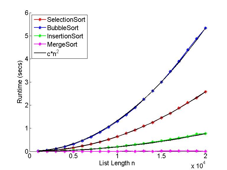
However, Big-O notation often describes the average or worst-case scenario. Let's look closer at the nuances.
Sorting Algorithms Time and Space Complexity | Sorting Algorithms | Big-O | Geekific
The video "Sorting Algorithms Time and Space Complexity" by Geekific provides a concise review of the time complexities for the algorithms we've covered.
Watch the following segments to refresh your memory on the time complexities: Bubble Sort: A simple but inefficient O(n^2) algorithm. Selection & Insertion Sort: Both are also O(n^2) in the average and worst case. Merge Sort: A detailed breakdown showing why it's consistently O(n \log n). You can skim this part as it recaps what we covered last lesson. Pay attention to how the analysis for Bubble, Selection, and Insertion Sort involves nested loops, leading to the n \times n or O(n^2) complexity.
An important detail the video touches on is the difference between best, average, and worst cases:
- Selection Sort: Always performs comparisons, regardless of the input data's order. It has no "best case" scenario that improves its complexity.
- Bubble and Insertion Sort: Have a best-case time complexity of . This occurs if the array is already sorted (or nearly sorted). In this situation, Bubble Sort makes one pass and stops, and Insertion Sort finds that each element is already in its correct position without needing to shift others.
- Merge Sort: Is a consistent performer. It is always , whether the data is sorted, reversed, or random. The process of dividing and merging doesn't change based on the input's order.
2. Space Complexity: The Memory Cost
Time isn't the only resource we care about; memory usage is also critical. Here we distinguish between algorithms that sort in-place versus those that are out-of-place.
- An in-place algorithm has a space complexity of . It sorts the data within the original array, using only a constant amount of extra memory for temporary variables (like for a swap).
- An out-of-place algorithm requires significant extra memory that scales with the input size, often .
Bubble, Selection, and Insertion Sort are all in-place algorithms. They work by swapping elements directly within the array.
Merge Sort, as we saw, is an out-of-place algorithm. Its merge step requires an auxiliary array to combine the sorted halves. The size of this temporary array can be up to n, leading to a space complexity of .
This illustrates a fundamental concept in computer science: the space-time trade-off. Merge Sort achieves its faster time complexity at the cost of using more memory. The simpler algorithms are slower but more memory-efficient.
The following video explains this trade-off and introduces another key concept: stability.
Explaining EVERY Sorting Algorithm (part 1)
Let's watch a segment from "Explaining EVERY Sorting Algorithm" by Kuvina Saydaki. This video provides excellent visualizations.
Watch the segment from stability and space. Focus on these three points: The definition of a stable sorting algorithm. The explanation of space complexity, confirming why Merge Sort is O(n) and the others are O(1) (it also mentions Quick Sort's O(\log n) space, which we will discuss later). The introduction to the space-time trade-off.
3. Stability: Preserving Relative Order
As you just saw, stability is another important characteristic. A stable sorting algorithm maintains the original relative order of elements that have equal values.
Why does this matter? Imagine you have a spreadsheet of customer data, which you've already sorted alphabetically by city. Now, you want to sort this list by country.
- If you use a stable sort, all customers within the same country (e.g., "USA") will remain sorted alphabetically by their city.
- If you use an unstable sort, the original city-based ordering might be lost.
Let's categorize our algorithms:
- Stable:
- Bubble Sort: Yes. It only swaps adjacent elements, so two equal elements will never leapfrog each other.
- Insertion Sort: Yes. It scans backwards and places an element, but never moves it past an equal element that came before it.
- Merge Sort: Yes. When merging, if elements from the left and right sub-arrays are equal, we can simply choose to take the element from the left sub-array first, preserving the original order.
- Unstable:
- Selection Sort: No. It finds the minimum element and swaps it with the element at the current position. This can involve a long-distance swap, moving the minimum element past other equal elements, thus changing their relative order.
4. Summary and Comparison
Let's consolidate everything into a single table. This is your high-level guide for comparing these four algorithms.
| Algorithm | Time Complexity (Best) | Time Complexity (Avg.) | Time Complexity (Worst) | Space Complexity (Worst) | Stability |
|---|---|---|---|---|---|
| Bubble Sort | Stable | ||||
| Selection Sort | Unstable | ||||
| Insertion Sort | Stable | ||||
| Merge Sort | Stable |
This table provides a dense summary of the trade-offs. You can find similar, more extensive tables in documentation that cover even more algorithms.
Analysis of different sorting techniques
The GeeksforGeeks article "Analysis of different sorting techniques" includes a comprehensive comparison table.
Take a look at the "Time and Space Complexity Comparison Table". You'll see our four algorithms listed among others. This reinforces the data in our table and shows you how other algorithms like Heap Sort and Quick Sort fit into the landscape.
5. Making the Right Choice: Practical Scenarios
Based on this analysis, when should you use each algorithm?
-
When to use Insertion Sort (or Bubble Sort)?
- When you know your data is small (e.g., n < 20). For small
n, the overhead of a complex algorithm like Merge Sort can make it slower than a simple algorithm. - When the data is almost sorted. Insertion Sort's best-case performance makes it extremely fast for tidying up a list with only a few misplaced elements.
- When you know your data is small (e.g., n < 20). For small
-
When to use Merge Sort?
- When you are sorting large datasets. Its time complexity is essential for performance.
- When you need guaranteed performance. The worst-case is the same as the average-case, so you are protected from catastrophic slowdowns on certain inputs.
- When stability is required.
- When you have enough available memory to tolerate its space complexity.
-
When to use Selection Sort?
- In modern practice, it's rarely the best choice. Its lack of a best-case improvement and its instability make it less practical than Insertion Sort. Its one niche advantage is that it minimizes the number of swaps, which could be relevant if writing to memory is an extremely expensive operation.
Conclusion
Congratulations on completing this module! You have not only learned to implement four sorting algorithms but can now critically evaluate and compare them like a professional software developer.
Key Takeaways:
- There is no single "best" sorting algorithm. The optimal choice is always a trade-off.
- Merge Sort is the clear winner for large, general-purpose sorting where performance and predictability are key, provided you can afford the space.
- Insertion Sort is an excellent choice for small datasets or nearly sorted data due to its simplicity and best-case performance.
- Bubble Sort and Selection Sort are primarily educational tools for introducing sorting concepts; they are rarely used in production code due to their poor average-case performance.
- The primary criteria for choosing an algorithm are time complexity ( vs. ), space complexity (in-place vs. out-of-place), and stability.
Preview of the Next Lesson:
We are now at a major turning point in the course. Having built a strong foundation in C programming and fundamental algorithms, we will now shift our focus to data structures. In the next module, you will learn about Stacks and Queues. These are two of the most fundamental data structures in computer science, acting as building blocks for everything from parsing expressions to managing tasks in an operating system.