Merge Sort: Time and Space Complexity

Welcome to the next lesson in our journey through recursion and sorting. In our previous sessions, you've implemented the mergeSort algorithm and explored the call stack mechanism that enables recursion. Today, we'll connect the structure of the mergeSort algorithm directly to its performance.

Our goal is to analyze why mergeSort is considered a highly efficient sorting algorithm. We will derive its time complexity of $O(n\log n)$ and its space complexity of $O(n)$. Understanding this analysis is fundamental to making informed decisions about which algorithm to use in different scenarios.

1. The Anatomy of Merge Sort's Complexity

As we've seen, mergeSort uses a "divide and conquer" strategy. Its performance is a direct result of this two-part process:

1. Divide: The recursive splitting of the array into halves.
2. Conquer: The merging of the sorted halves back together.

The time complexity $O(n\log n)$ is a product of these two parts: the log n comes from the "divide" step, and the n comes from the "conquer" step. Let's break down each one.

2. The "log n" Factor: The Power of Halving

The "divide" phase of mergeSort repeatedly splits the array in half until we have sub-arrays of size 1. The key question is: how many times can you split an array of size n in half before you're left with single elements?

This is a classic logarithmic problem. Think of searching for a word in a physical dictionary. You don't start from page one; you open it to the middle. Based on where your word is alphabetically, you discard half the book and repeat the process with the remaining half. The number of times you have to do this is very small compared to the total number of pages.

This is the essence of logarithmic complexity. The following article provides an excellent intuition for this concept.

In mergeSort, this process of halving the array creates a recursion tree. If our initial array has n elements, the number of levels in this tree—the number of sets of recursive calls we have to make—is ${\log }_{2}n$.

Let's see this visually. The following video demonstrates how an array of size 8 is split, resulting in ${\log }_{2}8=3$ levels of splits.

3. The "n" Factor: Work Done at Each Level

Now we know the "divide" step gives us $\log n$ levels of recursion. But how much work is done at each of these levels? This is where the "conquer" (or merge) step comes in.

At each level of the recursion tree, we perform several merge operations. For example, at the bottom level, we merge pairs of 1-element arrays. At the next level up, we merge pairs of 2-element arrays, and so on.

The critical insight is this: at every single level of the recursion tree, the total number of elements processed across all merge operations for that level is exactly n.

To understand why the work per level is $O(n)$, let's first analyze a single merge operation.

Since merging k elements takes $O(k)$ time, and every level of the recursion tree involves merging a total of n elements, the work done at each level is $O(n)$.

4. Putting It All Together: Time Complexity is $O(n\log n)$

We've now established the two key components:

1. There are $\log n$ levels of recursion (from the splitting).
2. Each level performs a total of $O(n)$ work (from the merging).

The total time complexity is simply the product of these two:

This relationship is perfectly captured by the classic recursion tree diagram for mergeSort.

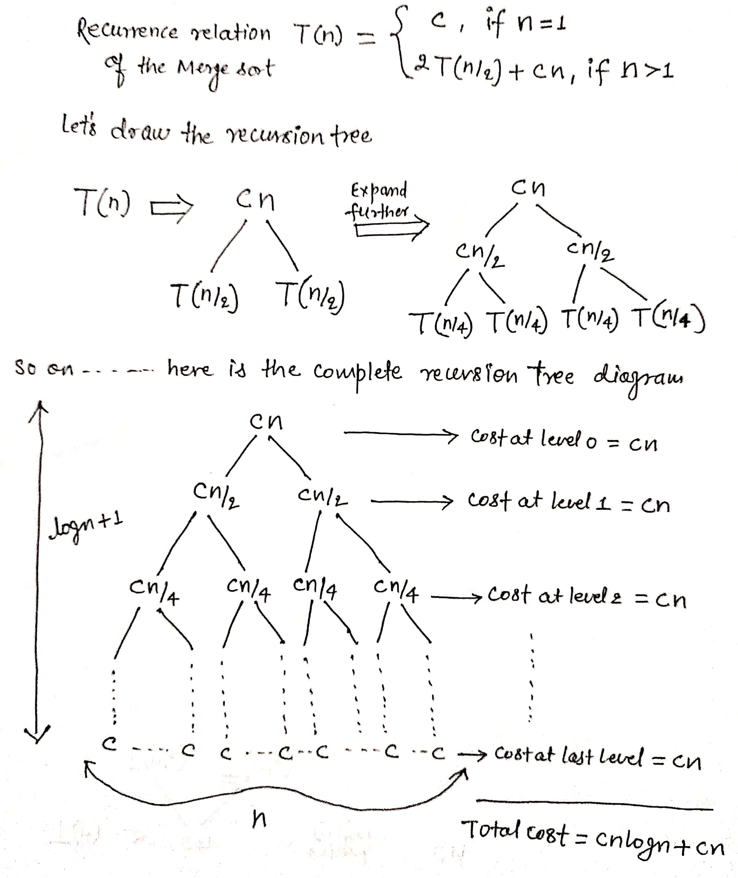
This also explains why mergeSort is so consistent. Whether the array is already sorted, in reverse order, or random, the algorithm still performs the same number of splits and merges. This is why its best-case, average-case, and worst-case time complexities are all $O(n\log n)$.

The Codecademy article below provides a great summary of this entire breakdown.

For those interested in a more formal mathematical proof, the following video section derives the exact formula for the number of comparisons, showing precisely where the $n\log n$ term originates. This is optional but can provide a deeper appreciation for the analysis.

5. Space Complexity: Where Does the Memory Go?

While mergeSort is excellent in terms of time, it comes at a cost: memory. Its space complexity is $O(n)$, which is less efficient than sorting algorithms like Selection Sort or Insertion Sort that operate "in-place" ($O(1)$ space).

There are two main contributors to mergeSort's memory usage:

1. The Auxiliary Array for Merging: As you saw in the merge function implementation, you need temporary storage to combine two sorted sub-arrays. To merge the final two halves of the main array (each of size n/2), you need a temporary array of size n. This is the dominant factor in memory usage, contributing $O(n)$ to the space complexity.

2. The Recursion Call Stack: In the last lesson, we saw how every recursive call adds a frame to the call stack. For mergeSort, the maximum depth of the recursion is the number of levels in our tree, which is $\log n$. Therefore, the call stack contributes $O(\log n)$ space.

When we combine these, the total space complexity is $O(n)+O(\log n)$. In Big-O notation, we drop the non-dominant terms, so the final space complexity simplifies to $O(n)$.

The following reading provides a concise explanation of this.

Conclusion

In this lesson, we've dissected the performance of the mergeSort algorithm. By analyzing its divide-and-conquer strategy, you can now explain precisely why its performance is so reliable and efficient.

Key Takeaways:

• Time Complexity is $O(n\log n)$: This is a product of having $\log n$ levels of recursion, with each level performing $O(n)$ work during the merge steps.
• Consistent Performance: mergeSort's time complexity is $O(n\log n)$ in the best, average, and worst cases because the number of divisions and merges is independent of the initial order of the data.
• Space Complexity is $O(n)$: This is dominated by the need for a temporary, auxiliary array of size n to perform the merge operations. The recursive call stack contributes a smaller $O(\log n)$ amount of space.

Preview of the Next Lesson:
You have now implemented and analyzed four different sorting algorithms: Bubble Sort, Selection Sort, Insertion Sort ($O(n^2)$), and Merge Sort ($O(n\log n)$). In our next lesson, we will bring it all together by comparing the performance characteristics of all of them. This will help you build the crucial skill of choosing the right tool for the job based on data size, memory constraints, and stability requirements.