Understanding Estimators: Properties and Definitions

Hello! Welcome to your next lesson on the theoretical foundations of AI.

In our last session, we explored the Law of Large Numbers (LLN) and the Central Limit Theorem (CLT). We saw that the sample mean, ${\bar{X}}_n$, not only converges to the true population mean $\mu$ (by the LLN) but also that its fluctuations around $\mu$ follow a normal distribution (by the CLT). In doing so, we informally described the sample mean as "unbiased" and "consistent."

Today, we will formalize these ideas. This lesson introduces the core concepts of statistical estimation. Your learning outcome is to define the concept of a statistical estimator and its properties (unbiasedness, consistency, and efficiency). Understanding these properties is crucial, as they provide the criteria we use to judge the quality of our machine learning models and statistical methods.

1. The Language of Estimation: Parameters, Estimators, and Estimates

Before we can evaluate estimators, we need to be precise about our terminology. In statistics, we distinguish between properties of the population (which are unknown) and quantities we calculate from our sample data.

A good starting point is this brief text, which lays out the essential vocabulary.

To summarize and build on that reading:

• Population Parameter ($\theta$): A fixed, but typically unknown, numerical characteristic of a population. Examples include the population mean ($\mu$), population variance (${\sigma }^2$), or the probability of success ($p$) in a Bernoulli trial.
• Estimator (${\hat{\theta }}_n$): A rule or function that tells us how to calculate an approximation of a parameter $\theta$ from the data in a random sample $(X_1,X_2,\dots ,X_n)$. Because it is a function of random variables, an estimator is itself a random variable. For example, the function ${\bar{X}}_n=\frac{1}{n}{\sum }_{i=1}^n{X}_i$ is an estimator for the parameter $\mu$.
• Estimate: A specific value of an estimator calculated from a particular, observed sample. An estimate is a fixed number. If you collect data and find your sample mean is 10.5, then 10.5 is your estimate of $\mu$.

In your past project on house price prediction, the true coefficients that relate square footage and location to price are the unknown parameters. The linear regression algorithm you used is the estimator. The specific coefficient values your model produced (e.g., "$150 per square foot") are the estimates.

2. Property 1: Unbiasedness

The first desirable property of an estimator is that it doesn't systematically over- or underestimate the true parameter. We want it to be correct "on average." This property is called unbiasedness.

The following video provides an excellent formal definition of an unbiased estimator and proves that the sample mean possesses this property.

As you saw, an estimator ${\hat{\theta }}_n$ is unbiased if its expected value is equal to the true parameter $\theta$. The expectation is taken over the sampling distribution of the estimator (i.e., over all possible samples of size $n$).

$\text{E}[{\hat{\theta }}_n]=\theta$

Let's formalize the proof from the video that the sample mean, ${\bar{X}}_n$, is an unbiased estimator for the population mean, $\mu$.
Given a random sample $X_1,\dots ,X_n$ where $\text{E}[X_i]=\mu$ for all $i$:

$$\begin{array}{rl}\text{E}[{\bar{X}}_n]& =\text{E}\left[\frac{1}{n}\sum _{i=1}^n{X}_i\right]\\ & =\frac{1}{n}\text{E}\left[\sum _{i=1}^n{X}_i\right]\text{(by linearity of expectation)}\\ & =\frac{1}{n}\sum _{i=1}^n\text{E}[X_i]\text{(by linearity of expectation)}\\ & =\frac{1}{n}\sum _{i=1}^n\mu \\ & =\frac{1}{n}(n\mu )\\ & =\mu \end{array}$$

Thus, we have proven that ${\bar{X}}_n$ is an unbiased estimator of $\mu$.

It is important to note that not all intuitive estimators are unbiased. For example, the estimator for population variance using a denominator of $n$, $S_n^2=\frac{1}{n}\sum (X_i-{\bar{X}}_n{)}^2$, is a biased estimator of ${\sigma }^2$. It can be shown that $\text{E}[S_n^2]=\frac{n-1}{n}{\sigma }^2$, which systematically underestimates the true variance. This is precisely why the sample variance is defined with a denominator of $n-1$.

3. Property 2: Consistency

An unbiased estimator is correct on average, but for any single sample, it might still be far from the true value. A consistent estimator is one that gets closer to the true parameter value as we collect more data.

This idea should sound familiar. It's the same concept of convergence in probability that we discussed in the last lesson with the Weak Law of Large Numbers.

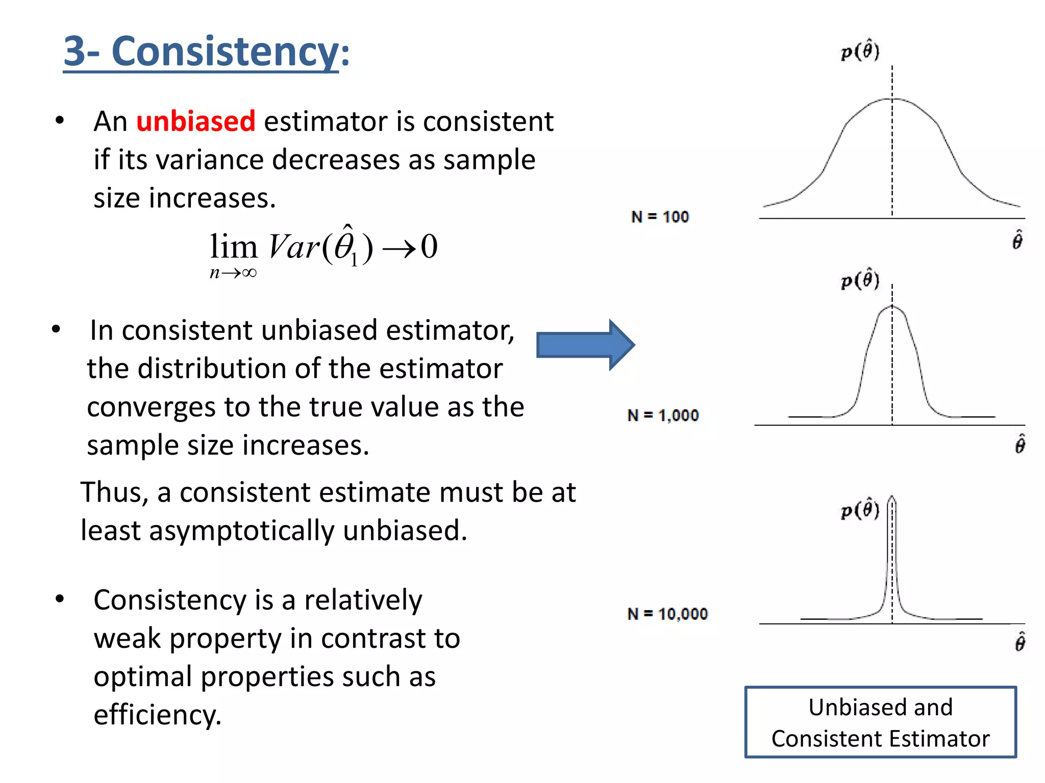
Formally, an estimator ${\hat{\theta }}_n$ is consistent if it converges in probability to $\theta$:
${\lim }_{n\to \infty }P(|{\hat{\theta }}_n-\theta |>ϵ)=0\text{for any }ϵ>0$

Proving this directly from the definition can be complex. Fortunately, there is a set of sufficient conditions that are often easier to check. This next video will introduce these conditions and use them to prove the consistency of the sample mean.

As the video explained, a sufficient (but not necessary) condition for an estimator ${\hat{\theta }}_n$ to be consistent is that its bias and variance both approach zero as $n\to \infty$.

1. Asymptotically Unbiased: ${\lim }_{n\to \infty }\text{E}[{\hat{\theta }}_n]=\theta$
2. Vanishing Variance: ${\lim }_{n\to \infty }\text{var}({\hat{\theta }}_n)=0$

Let's apply these conditions to the sample mean ${\bar{X}}_n$:

1. We already proved it is unbiased: $\text{E}[{\bar{X}}_n]=\mu$. This means it is also asymptotically unbiased since the limit is trivially $\mu$.
2. In the last lesson, we derived its variance: $\text{var}({\bar{X}}_n)=\frac{{\sigma }^2}{n}$. Taking the limit:
   ${\lim }_{n\to \infty }\text{var}({\bar{X}}_n)={\lim }_{n\to \infty }\frac{{\sigma }^2}{n}=0$

Since both conditions are met, the sample mean ${\bar{X}}_n$ is a consistent estimator of the population mean $\mu$.

Test your understanding!

Consider two estimators for a parameter $\theta$.

• Estimator A is unbiased, but its variance stays constant at 0.5, regardless of the sample size $n$.
• Estimator B has a bias of $10/n$, and its variance is $1/\sqrt{n}$.

Which of these estimators is consistent? Which is unbiased?

Show answer

• Estimator A: It is unbiased by definition. However, its variance does not approach 0 as $n\to \infty$. Therefore, it is not consistent.
• Estimator B: It is biased for any finite $n$. However, its bias ${\lim }_{n\to \infty }10/n=0$, so it is asymptotically unbiased. Its variance also approaches zero: ${\lim }_{n\to \infty }1/\sqrt{n}=0$. Since both sufficient conditions are met, Estimator B is consistent.

This shows that an estimator can be consistent without being unbiased for finite samples.

4. Property 3: Efficiency

Often, we may have several estimators that are both unbiased and consistent. How do we choose between them? Intuitively, we should prefer the estimator that is more "precise"—the one whose sampling distribution is more tightly packed around the true parameter. This concept is captured by efficiency.

An unbiased estimator ${\hat{\theta }}_A$ is said to be more efficient than another unbiased estimator ${\hat{\theta }}_B$ if its variance is smaller:
$\text{var}({\hat{\theta }}_A)<\text{var}({\hat{\theta }}_B)$

This leads to the idea of a "best" unbiased estimator: the Minimum Variance Unbiased Estimator (MVUE). But how can we know if an estimator has the minimum possible variance among all possible unbiased estimators?

The answer lies in a powerful result called the Cramér-Rao Lower Bound (CRLB). The CRLB provides a theoretical floor on the variance of any unbiased estimator.

This reading explains the concept of MVUE and introduces the CRLB.

As the text states, the Cramér-Rao Lower Bound establishes that for any unbiased estimator ${\hat{\theta }}_n$ of a parameter $\theta$, based on a sample of size $n$, its variance must satisfy:

$\text{var}({\hat{\theta }}_n)\ge \frac{1}{nI(\theta )}$

The term $I(\theta )$ is the Fisher Information, which measures how much information a single observation $X$ provides about the parameter $\theta$. It is defined as:
$I(\theta )=\text{E}\left[{\left(\frac{\partial }{\partial \theta }\log f(X;\theta )\right)}^2\right]$
where $f(X;\theta )$ is the probability density/mass function of the data.

An unbiased estimator that achieves this lower bound (i.e., its variance equals the CRLB) is called an efficient estimator, and it is the MVUE.

A Broader View: The Bias-Variance Tradeoff

Focusing solely on unbiasedness can sometimes be limiting. A slightly biased estimator might be preferable if its variance is drastically lower. This introduces the famous bias-variance tradeoff. A useful metric that combines both bias and variance is the Mean Squared Error (MSE).

The MSE of an estimator $\hat{\theta }$ is defined as the expected squared difference between the estimator and the true parameter:
$\text{MSE}(\hat{\theta })=\text{E}[(\hat{\theta }-\theta {)}^2]$

Crucially, the MSE can be decomposed into two components: the variance of the estimator and its squared bias. The derivation is as follows:

Let $\text{Bias}(\hat{\theta })=\text{E}[\hat{\theta }]-\theta$.

$$\begin{array}{rl}\text{MSE}(\hat{\theta })& =\text{E}[(\hat{\theta }-\theta {)}^2]\\ & =\text{E}[(\hat{\theta }-\text{E}[\hat{\theta }]+\text{E}[\hat{\theta }]-\theta {)}^2]\\ & =\text{E}[(\underset{\text{deviation from mean}}{\underbrace{\hat{\theta }-\text{E}[\hat{\theta }]}})+(\underset{\text{Bias}}{\underbrace{\text{E}[\hat{\theta }]-\theta }}){]}^2\\ & =\text{E}[(\hat{\theta }-\text{E}[\hat{\theta }]{)}^2+2(\hat{\theta }-\text{E}[\hat{\theta }])(\text{Bias})+(\text{Bias}{)}^2]\\ & =\text{E}[(\hat{\theta }-\text{E}[\hat{\theta }]{)}^2]+2(\text{Bias})\text{E}[\hat{\theta }-\text{E}[\hat{\theta }]]+\text{E}[(\text{Bias}{)}^2]\end{array}$$

The first term is the definition of variance, $\text{var}(\hat{\theta })$. The middle term is zero because $\text{E}[\hat{\theta }-\text{E}[\hat{\theta }]]=\text{E}[\hat{\theta }]-\text{E}[\hat{\theta }]=0$. The last term is $(\text{Bias}{)}^2$ since Bias is a constant. This gives the famous decomposition:

$\text{MSE}(\hat{\theta })=\text{var}(\hat{\theta })+[\text{Bias}(\hat{\theta }){]}^2$

This equation is fundamental in machine learning. It tells us that an estimator's total error is a sum of its variance (how much the estimate varies from sample to sample) and its squared bias (how far off it is on average). Many advanced techniques, such as regularization in regression, intentionally introduce a small amount of bias to significantly reduce variance, thereby lowering the overall MSE.

Conclusion

Today, we have established a formal framework for evaluating statistical estimators. These concepts are the bedrock of statistical inference and model evaluation in machine learning.

Key Takeaways:

• An estimator is a function of sample data used to approximate an unknown population parameter.
• Unbiasedness means an estimator is correct on average ($\text{E}[\hat{\theta }]=\theta$).
• Consistency means an estimator converges to the true parameter as the sample size increases. This can be proven if the estimator is asymptotically unbiased and its variance vanishes.
• Efficiency refers to the precision of an estimator. For unbiased estimators, the most efficient is the MVUE, which has the lowest possible variance, as defined by the Cramér-Rao Lower Bound.
• The Mean Squared Error (MSE) provides a complete picture of an estimator's quality by combining its variance and bias.

Preview of the Next Lesson:
We now know the properties of a good estimator. But this begs the question: how do we find good estimators in the first place? In our next lesson, we will begin to answer that by deriving the Principle of Maximum Likelihood Estimation (MLE), a powerful and general method for constructing high-quality estimators for almost any statistical model.