Law of Large Numbers and Central Limit Theorem

Hello! Welcome to your next lesson in our journey through the mathematical foundations of AI.

In our previous lessons, we've built a solid toolkit for describing random variables and their relationships using concepts like expected value, variance, and covariance. Now, we are going to ask a different, more profound question: what happens when we observe and average many random events? This question lies at the heart of all statistical inference and machine learning—it's how we learn from data.

Today, we will explore two of the most celebrated and fundamental theorems in probability theory: the Law of Large Numbers (LLN) and the Central Limit Theorem (CLT). Your learning outcome is to state the Law of Large Numbers (LLN) and the Central Limit Theorem (CLT) and explain their implications for statistical inference. These theorems provide the theoretical bedrock for why we can be confident that our statistical and machine learning models learn meaningful patterns from data.

1. The Setup: Averaging Random Variables

Both the LLN and the CLT deal with the behavior of the sample mean. Imagine we have a set of $n$ random variables, $X_1,X_2,\dots ,X_n$, that are independent and identically distributed (i.i.d.). This is a standard assumption in many statistical models, representing repeated, independent experiments of the same underlying phenomenon (e.g., flipping the same coin $n$ times, or drawing $n$ data points from the same population).

Let's assume each $X_i$ has a true (population) mean $\mu$ and a finite variance ${\sigma }^2$. The sample mean is defined as:

${\bar{X}}_n=\frac{1}{n}{\sum }_{i=1}^n{X}_i$

The central question for today is: what can we say about ${\bar{X}}_n$ as our sample size $n$ gets very large?

2. The Law of Large Numbers: Convergence to the Truth

The Law of Large Numbers (LLN) provides the first part of the answer. Intuitively, it states that as you collect more and more data, the sample mean will get closer and closer to the true population mean. It's the mathematical guarantee behind the "wisdom of the crowd."

To formalize this, we need to understand different types of convergence for random variables. The following video provides a fantastic introduction to the LLN, distinguishes between the "strong" and "weak" versions of the law, and offers a rigorous proof for the Weak Law of Large Numbers (WLLN).

2.1 Formal Statement and Proof of the WLLN

As you saw in the video, the Weak Law of Large Numbers (WLLN) states that the sample mean ${\bar{X}}_n$ converges in probability to the true mean $\mu$. Formally, for any small positive number $ϵ$, the probability that the sample mean is further away from the true mean than $ϵ$ approaches zero as the sample size $n$ goes to infinity.

${\lim }_{n\to \infty }P(|{\bar{X}}_n-\mu |>ϵ)=0$

The proof you saw is elegant and brings together several concepts we've studied. Let's recap the steps:

1. Find the Expected Value and Variance of the Sample Mean:

   • $\text{E}[{\bar{X}}_n]=\text{E}\left[\frac{1}{n}\sum X_i\right]=\frac{1}{n}\sum \text{E}[X_i]=\frac{1}{n}(n\mu )=\mu$. The sample mean is an unbiased estimator of the population mean.
   • $\text{var}({\bar{X}}_n)=\text{var}\left(\frac{1}{n}\sum X_i\right)=\frac{1}{n^2}\text{var}(\sum X_i)$. Since the $X_i$ are independent, the variance of the sum is the sum of the variances: $\frac{1}{n^2}\sum \text{var}(X_i)=\frac{1}{n^2}(n{\sigma }^2)=\frac{{\sigma }^2}{n}$.

2. Apply Chebyshev's Inequality:
   Chebyshev's inequality states for a random variable $Y$ with mean ${\mu }_Y$ and variance ${\sigma }_Y^2$: $P(|Y-{\mu }_Y|\ge k)\le \frac{{\sigma }_Y^2}{k^2}$.
   Let's apply this to ${\bar{X}}_n$, where its mean is $\mu$ and its variance is ${\sigma }^2/n$. We set our threshold $k=ϵ$:
   $P(|{\bar{X}}_n-\mu |\ge ϵ)\le \frac{\text{var}({\bar{X}}_n)}{{ϵ}^2}=\frac{{\sigma }^2/n}{{ϵ}^2}=\frac{{\sigma }^2}{n{ϵ}^2}$

3. Take the Limit:
   As $n\to \infty$, the right-hand side $\frac{{\sigma }^2}{n{ϵ}^2}$ clearly goes to 0.
   ${\lim }_{n\to \infty }P(|{\bar{X}}_n-\mu |\ge ϵ)=0$
   This completes the proof.

The video also mentioned the Strong Law of Large Numbers (SLLN), which makes a stronger claim: $P({\lim }_{n\to \infty }{\bar{X}}_n=\mu )=1$. This means that for any single, infinitely long experiment, the sequence of sample means is guaranteed to converge to $\mu$. The weak law only says that for a large but finite $n$, being far from the mean is unlikely. For our purposes, the implications are very similar.

2.2 Implications of the LLN for Inference

The LLN is the foundational principle that makes statistical estimation possible.

• It justifies using sample statistics to estimate population parameters. For instance, the reason we use the proportion of heads in a large number of coin flips to estimate the coin's true bias is a direct consequence of the LLN.
• It guarantees consistency. In statistical estimation theory (which we will cover next), an estimator is called consistent if it converges to the true value of the parameter as the sample size grows. The LLN proves that the sample mean is a consistent estimator for the population mean.

3. The Central Limit Theorem: The Shape of the Fluctuation

The LLN tells us that the sample mean ${\bar{X}}_n$ converges to the constant $\mu$. But this doesn't tell us anything about the distribution of ${\bar{X}}_n$ for a large but finite $n$. How does it fluctuate around $\mu$? The Central Limit Theorem (CLT) provides the remarkable answer.

The CLT states that the distribution of the (properly standardized) sample mean approaches a normal distribution as the sample size increases, regardless of the original distribution of the data. This is arguably the most important theorem in all of statistics.

Let's return to the Harvard video to understand the statement and the rigorous proof of this theorem.

3.1 Formal Statement of the CLT

As the video proved, the Central Limit Theorem states that if $X_1,\dots ,X_n$ are i.i.d. random variables with mean $\mu$ and finite variance ${\sigma }^2$, then the standardized sample mean converges in distribution to a standard normal distribution:

$Z_n=\frac{{\bar{X}}_n-\mu }{\sigma /\sqrt{n}}\stackrel{d}{\to }N(0,1)\text{as }n\to \infty$

Here, $\stackrel{d}{\to }$ denotes convergence in distribution. This means the CDF of $Z_n$ approaches the CDF of the standard normal distribution.

Equivalently, it's often written in terms of the sum $S_n=\sum X_i$, which has mean $n\mu$ and variance $n{\sigma }^2$:
$\frac{S_n-n\mu }{\sigma \sqrt{n}}\stackrel{d}{\to }N(0,1)\text{as }n\to \infty$

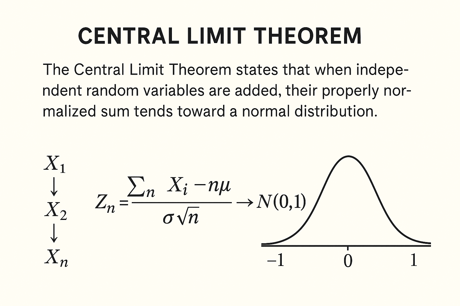
The truly amazing part is that this holds true whether the original $X_i$s come from a Bernoulli, Poisson, Exponential, or some other complex distribution, as long as the variance is finite.

3.2 Implications of the CLT for Inference

The practical power of the CLT is immense. It is the engine behind most of frequentist statistical inference, particularly hypothesis testing and confidence intervals.

To see exactly how, let's explore how the CLT is used to create "asymptotic pivots," which are quantities we can use to make inferences.

As the reading explains, the CLT allows us to make probabilistic statements about our sample mean. Because we know that for a large $n$, $\frac{{\bar{X}}_n-\mu }{\sigma /\sqrt{n}}$ is approximately distributed as $N(0,1)$, we can use the properties of the standard normal distribution to calculate probabilities and construct confidence intervals.

For example, we know that for a standard normal variable $Z$, $P(-1.96\le Z\le 1.96)\approx 0.95$. By the CLT, this means:
$P\left(-1.96\le \frac{{\bar{X}}_n-\mu }{\sigma /\sqrt{n}}\le 1.96\right)\approx 0.95$
Rearranging this inequality allows us to form an approximate 95% confidence interval for the unknown population mean $\mu$:
${\bar{X}}_n\pm 1.96\frac{\sigma }{\sqrt{n}}$
This is a cornerstone of statistical inference. Even if $\sigma$ is unknown, for large $n$ we can substitute the sample standard deviation $s$ without changing the result much.

The CLT also justifies the use of normal approximations for other distributions, like the binomial and Poisson, when $n$ is large. The Harvard video demonstrated this with the normal approximation to the binomial, a very common and powerful application.

Conclusion

In this lesson, we have explored two pillars of probability theory that bridge the gap between theory and practice. They explain why we can be confident in learning from data.

Key Takeaways:

• The Law of Large Numbers (LLN): States that the sample mean ${\bar{X}}_n$ converges to the population mean $\mu$ as the sample size $n$ grows. This provides the justification for estimation.
• The Central Limit Theorem (CLT): States that the distribution of the standardized sample mean $\frac{{\bar{X}}_n-\mu }{\sigma /\sqrt{n}}$ converges to a standard normal distribution $N(0,1)$, regardless of the original data's distribution. This is the foundation for hypothesis testing and constructing confidence intervals.
• In short: The LLN tells us where the sample average is going (the true mean), and the CLT tells us the path it takes to get there (it follows a normal distribution).

Preview of the Next Lesson:
With the LLN and CLT as our theoretical foundation, we are now perfectly positioned to formalize the process of estimation. In the next lesson, we will begin our module on Statistical Estimation Theory. We will define what a statistical "estimator" is and introduce the key criteria for judging its quality, such as unbiasedness, consistency (which you now know is guaranteed for the sample mean by the LLN), and efficiency.