Building Scaled Dot-Product Attention in Python

Introduction

In our previous lesson, you successfully traced the complete data flow through a Transformer encoder block. You now have a high-level, architectural understanding of how multi-head attention, residual connections, and layer normalization work together to transform input embeddings into rich, contextual representations.

Today, we transition from this architectural blueprint to the fundamental engine that powers it. Our focus is to implement the core mechanism of scaled dot-product attention from scratch. We will build a single, functional self-attention head in Python, translating the mathematical formula we've discussed into tangible code. This is a critical hands-on step that moves us from 'what' the components are to 'how' they actually compute. For someone with your interest in systems engineering, understanding this implementation from first principles is key to grasping the performance and computational characteristics of the entire Transformer model.

The Mathematical Blueprint of Attention

At the heart of self-attention lies a single, elegant formula. All the complexity of the mechanism can be derived from understanding its parts.

Let's deconstruct this. The process takes an input sequence of token embeddings, represented by a matrix $X$ of shape (seq_len, d_model), and transforms it through five distinct steps:

1. Projection into Q, K, V spaces: The input embeddings $X$ are projected using three separate, learnable weight matrices ($W_Q$, $W_K$, $W_V$) to create the Query, Key, and Value matrices.

   $$Q=X{W}_Q,K=X{W}_K,V=X{W}_V$$

   These projections allow the model to learn to transform the same input embedding into three different roles. The Query represents the current token's "question" about other tokens. The Key represents each token's "label" or "identity" that queries can match against. The Value represents the actual content or information of each token to be retrieved.

2. Calculate Similarity Scores: The dot product between the Query matrix and the transpose of the Key matrix ($Q{K}^T$) is computed. Recalling from our linear algebra module, the dot product measures similarity or alignment. The resulting matrix, often called the compatibility or scores matrix, contains a score for how much each token (query) should attend to every other token (key).

3. Scale for Stability: The scores are scaled by dividing by the square root of the dimension of the key vectors, $\sqrt{d_k}$. As we discussed, this prevents the dot product values from becoming excessively large, which would push the subsequent softmax function into regions with near-zero gradients, hindering learning.

4. Normalize with Softmax: The softmax function is applied to each row of the scaled scores matrix. This converts the raw similarity scores into a probability distribution—the attention weights. Each row now sums to 1, indicating what percentage of "attention" a given token should pay to all other tokens in the sequence.

5. Compute the Weighted Sum: Finally, the attention weights matrix is multiplied by the Value matrix $V$. This produces the output for each token as a weighted sum of all other tokens' values, where the weights are determined by the attention scores.

To see these steps animated, the following video provides a clear, step-by-step walkthrough.

From Blueprint to Code: Implementing a Self-Attention Head

Now, let's translate this mathematical process into a Python implementation using NumPy. We will construct a class for a single self-attention head. This single head is the building block that gets replicated in the full multi-head attention mechanism.

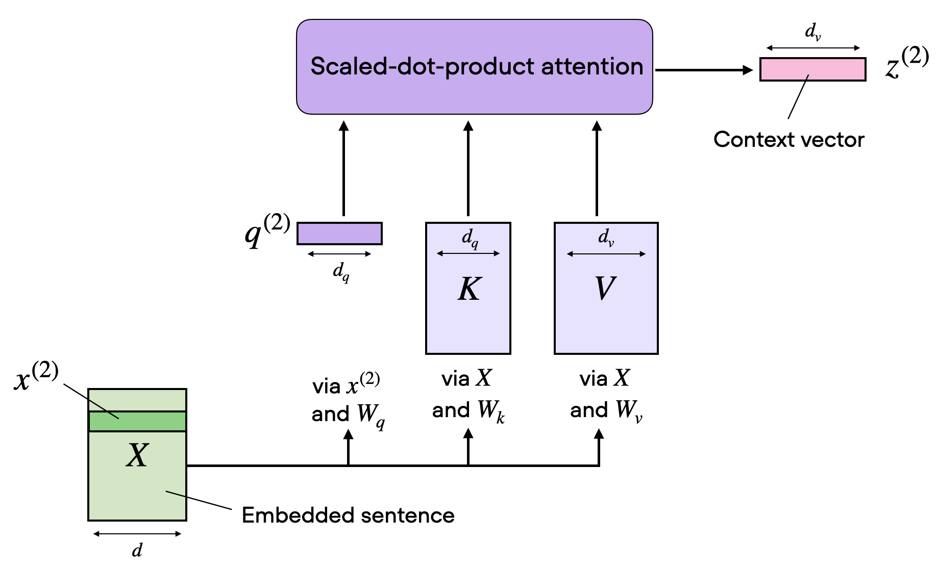
This diagram shows the data flow for a single attention head processing one token's query $q^{(2)}$ against all keys (K) and values (V) from the input sentence X. Our implementation will do this for all tokens in the sequence simultaneously using matrix operations.

We'll follow the clear, shape-focused implementation style outlined in Eli Bendersky's excellent notes.

Let's build this step-by-step.

import numpy as np

def softmax(x, axis=-1):
    """Numerically stable softmax function."""
    # Subtract the max for numerical stability
    e_x = np.exp(x - np.max(x, axis=axis, keepdims=True))
    # Divide by sums across last dimension
    return e_x / np.sum(e_x, axis=axis, keepdims=True)

class SingleHeadSelfAttention:
    def __init__(self, d_model, d_head):
        """
        Initializes a single self-attention head.
        
        Args:
            d_model (int): The dimensionality of the input token embeddings.
            d_head (int): The dimensionality of the query, key, and value vectors.
        """
        self.d_model = d_model
        self.d_head = d_head
        
        # Initialize learnable weight matrices
        # In a real framework, these would be initialized and tracked for gradients.
        # Here, we use random values for demonstration.
        self.W_q = np.random.randn(d_model, d_head)
        self.W_k = np.random.randn(d_model, d_head)
        self.W_v = np.random.randn(d_model, d_head)

    def forward(self, x):
        """
        Performs the forward pass for the self-attention head.
        
        Args:
            x (np.ndarray): Input tensor of shape (seq_len, d_model).
            
        Returns:
            np.ndarray: Output tensor of shape (seq_len, d_head).
        """
        seq_len, d_model = x.shape
        
        # 1. Project inputs into Q, K, V spaces
        # (seq_len, d_model) @ (d_model, d_head) -> (seq_len, d_head)
        q = x @ self.W_q
        k = x @ self.W_k
        v = x @ self.W_v
        
        # 2. Calculate similarity scores
        # (seq_len, d_head) @ (d_head, seq_len) -> (seq_len, seq_len)
        scores = q @ k.T
        
        # 3. Scale for stability
        scaled_scores = scores / np.sqrt(self.d_head)
        
        # 4. Normalize with softmax to get attention weights
        # The result is a (seq_len, seq_len) matrix where each row sums to 1.
        attention_weights = softmax(scaled_scores, axis=-1)
        
        # 5. Compute the weighted sum of Value vectors
        # (seq_len, seq_len) @ (seq_len, d_head) -> (seq_len, d_head)
        output = attention_weights @ v
        
        return output, attention_weights # Also returning weights for visualization

To test our implementation:

# --- Configuration ---
seq_len = 5       # Number of tokens in the sequence
d_model = 128     # Dimension of token embeddings
d_head = 64       # Dimension of Q, K, V vectors for this head

# --- Create dummy input ---
# A batch of one sequence with 5 tokens, each of 128 dimensions.
x_input = np.random.randn(seq_len, d_model)

# --- Instantiate and run the attention head ---
attention_head = SingleHeadSelfAttention(d_model, d_head)
output, weights = attention_head.forward(x_input)

# --- Check the shapes ---
print("Input shape:", x_input.shape)
print("Output shape:", output.shape)
print("Attention weights shape:", weights.shape)
print("\nFirst row of attention weights (sums to 1):", weights[0])
print("Sum of first row:", np.sum(weights[0]))

The output of this code will confirm that our input of shape (5, 128) is transformed into an output of shape (5, 64), which is the contextualized representation produced by this single head.

An Important Detail: Masking

The implementation above allows every token to attend to every other token, including those that come later in the sequence. This is perfectly fine for the encoder of a Transformer (like in BERT), which processes the entire input sentence at once.

However, for a decoder (like in GPT) that generates text one token at a time, we must prevent the model from "cheating" by looking at future tokens. This is achieved through masking.

The idea is simple: before applying the softmax function, we add a very large negative number (negative infinity) to the attention scores for all positions that should be ignored. When softmax is applied, $e^{-\infty }$ becomes 0, effectively nullifying the attention to those future positions.

We can add an optional mask argument to our forward method:

# (Inside the SingleHeadSelfAttention class)
def forward(self, x, mask=None):
    # ... (Q, K, V projection and score calculation are the same)
    
    scaled_scores = scores / np.sqrt(self.d_head)
    
    # --- ADD MASKING STEP ---
    if mask is not None:
        # Where mask is 0, set scores to a large negative number.
        scaled_scores = np.where(mask == 0, -np.inf, scaled_scores)

    attention_weights = softmax(scaled_scores, axis=-1)
    output = attention_weights @ v
    
    return output, attention_weights

To use this for auto-regressive decoding, you would create a "look-ahead" mask, which is a lower-triangular matrix of ones.

# Create a look-ahead mask for a sequence of length 5
look_ahead_mask = np.tril(np.ones((seq_len, seq_len)))
print("\nLook-ahead mask:\n", look_ahead_mask)

# Run with the mask
output_masked, weights_masked = attention_head.forward(x_input, mask=look_ahead_mask)

# The upper triangle of the weights matrix will now be zero
print("\nMasked attention weights (first 3x3):\n", weights_masked[:3, :3])

Conclusion

In this lesson, you have moved from a theoretical understanding of the Transformer architecture to a practical, low-level implementation of its core component. By building a self-attention head from scratch, you have solidified your grasp of how inputs are projected, similarities are scored, and contextual outputs are computed.

Key Takeaways:

• Scaled Dot-Product Attention is a sequence of matrix operations: Projection ($Q,K,V$), Score ($Q{K}^T$), Scale ($/\sqrt{d_k}$), Normalize (Softmax), and Weighted Sum ($\cdot V$).
• The learnable weight matrices $W_Q,W_K,W_V$ are what allow the model to learn meaningful projections for querying and retrieving information.
• Tensor shapes are critical. We transformed an input of (seq_len, d_model) into an output of (seq_len, d_head).
• Masking is an essential addition for auto-regressive models (like decoders) to enforce causality and prevent the model from attending to future tokens. It's implemented by adding negative infinity to scores before the softmax.

Preview of the Next Lesson:
While a single attention head is powerful, it can only learn one type of relationship between tokens. The true power of Transformers comes from multi-head attention. In our next lesson, we will parallelize our single-head implementation to build a full multi-head attention layer. We will explore how running multiple heads allows the model to capture diverse syntactic and semantic relationships simultaneously and discuss the efficient, vectorized implementation that makes it practical. You will see how the outputs from all heads are concatenated and projected to produce the final output of the sub-layer, as depicted in the diagram below.

A preview of the multi-head attention mechanism. Multiple attention heads compute in parallel, and their outputs are concatenated and projected to form the final output.