Autoencoders: Architecture, Dimensionality Reduction, and Representation Learning

Introduction

Welcome to our new module on generative modeling. In the previous module, we culminated our study of Transformers by implementing the scaled dot-product attention mechanism. You saw how input data could be transformed into different representations—Query, Key, and Value—to compute rich, contextual embeddings. This idea of learning powerful representations is a central theme in deep learning, and today, we will explore it from a different perspective: compression and reconstruction.

Our goal for this lesson is to understand the architecture and purpose of autoencoders. These are neural networks designed for unsupervised representation learning, often by performing dimensionality reduction. Following your preferred learning protocol, we will first ground our discussion in its classical machine learning ancestor: Principal Component Analysis (PCA). By understanding the limitations of this linear method, you will appreciate why the non-linear capabilities of autoencoders are so powerful, especially for the complex, high-dimensional data we encounter in computer graphics.

The Classical Precursor: Linear Dimensionality Reduction with PCA

In Module 2, we touched upon PCA as an application of eigendecomposition. At its core, PCA is a technique for dimensionality reduction that identifies the directions of maximum variance in a dataset. It projects the data onto a lower-dimensional linear subspace—a hyperplane—spanned by a set of orthogonal axes called principal components.

The key word here is linear. PCA is exceptionally good at reducing dimensionality when the important structure in the data can be captured by a flat plane. But what if it can't?

Consider data that lies on a curved manifold, like a spiral or the surface of a sphere. A linear projection onto a plane would fail to preserve the intrinsic structure of the data, potentially mapping distant points on the manifold close together in the projection.

This leads to our first question: Imagine you have a 3D point cloud of a coiled rope. If you use PCA to project this data down to 2D, what would the resulting representation look like, and what crucial information about the rope's structure would be lost?

The limitation you're contemplating is precisely where PCA falters. A 2D plane cannot effectively "unroll" the coil; it can only squash it flat, losing the information about its helical structure.

To capture such complex, non-linear structures, we need a more powerful, non-linear approach. This is the motivation for autoencoders.

The Autoencoder: A Non-Linear Generalization

An autoencoder is a type of artificial neural network used to learn efficient data codings in an unsupervised manner. The aim is to learn a representation (encoding) for a set of data, typically for dimensionality reduction, by training the network to ignore signal "noise".

The architecture is conceptually simple and consists of two main parts connected by a bottleneck:

1. The Encoder: This part of the network compresses the input into a low-dimensional latent-space representation. We can denote the encoder as a function $z=g_{\varphi }(x)$, where $x$ is the input and $\varphi$ are the parameters (weights and biases) of the encoder.
2. The Decoder: This part of the network reconstructs the input from the latent-space representation. We can denote the decoder as $\hat{x}=f_{\theta }(z)$, where $\theta$ are the parameters of the decoder.

The central component connecting them is the bottleneck, which is the hidden layer that contains the compressed representation $z$. This layer has fewer neurons than the input/output layers, forcing the network to learn a compressed representation of the data.

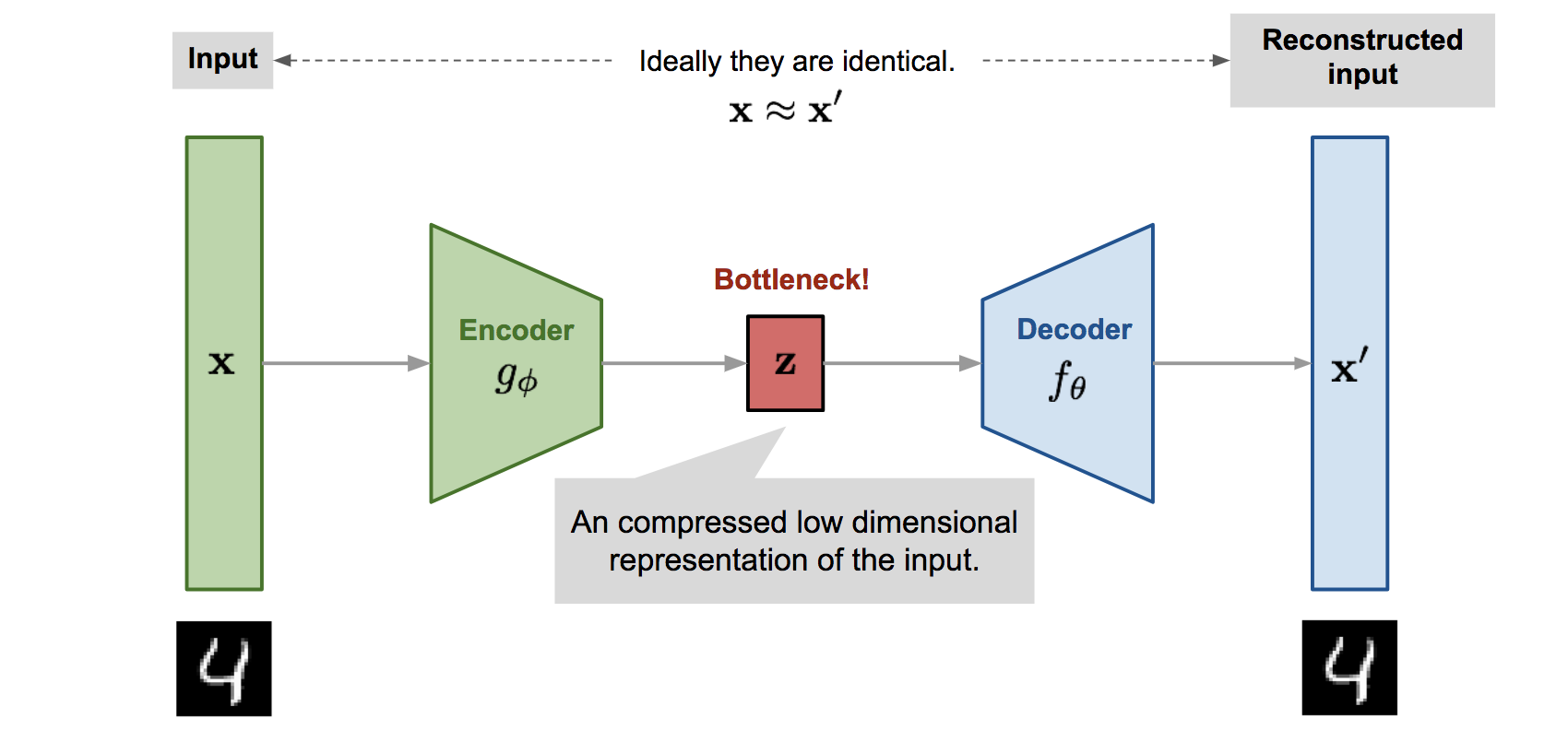
The network is trained by minimizing a reconstruction loss, $L(x,\hat{x})$, which measures the difference between the original input $x$ and the reconstructed output $\hat{x}$. In essence, the autoencoder is learning an approximation of the identity function, but its architecture prevents it from learning a trivial solution.

Let's watch a short video that formalizes this structure.

Undercomplete vs. Overcomplete Autoencoders

The dimensionality of the bottleneck layer relative to the input is a critical design choice.

• Undercomplete Autoencoder: When the dimension of the latent space $z$ is less than the dimension of the input $x$, the autoencoder is undercomplete. The bottleneck forces the network to select and learn the most salient features of the input data. This is the standard setup for dimensionality reduction and is directly analogous to PCA's goal.

• Overcomplete Autoencoder: If the latent space dimension is greater than or equal to the input dimension, it's an overcomplete autoencoder. This poses a challenge. Consider this: If the bottleneck is as large as the input, what trivial (and useless) strategy could the network learn to achieve a perfect, zero-loss reconstruction?

The network could simply learn to copy the input values directly through the bottleneck to the output, creating a perfect identity function without learning any meaningful underlying structure. To make overcomplete autoencoders useful, they must be regularized (e.g., by enforcing sparsity in the bottleneck activations), which forces them to learn interesting structures even with the added capacity.

Let's continue with the video to solidify this distinction.

The Role of Activation Functions and Loss Functions

Just like any other neural network, the choice of activation functions and the loss function is crucial and depends on the properties of your data. Let's consider two common scenarios for image data, where pixel values are often normalized to the range [0, 1].

Case 1: Real-Valued Inputs and MSE Loss

When inputs are continuous values (like normalized pixel intensities), a common setup is:

• Encoder Activation: A non-linear activation like ReLU is typical.
• Decoder Output Activation: A Sigmoid function is often used to ensure the output values are in the same [0, 1] range as the input. If the input data isn't normalized, a linear activation might be used.
• Loss Function: The Mean Squared Error (MSE) is a natural choice. It measures the average squared difference between the input and reconstructed pixels. $$L_{\text{MSE}}(x,\hat{x})=\frac{1}{N}\sum _{i=1}^N(x_i-{\hat{x}}_i{)}^2$$

Case 2: Binary Inputs and Cross-Entropy Loss

If we treat each pixel as a binary random variable (either 0 or 1), we can take a more probabilistic approach.

• Decoder Output Activation: A Sigmoid activation is used, but its output is interpreted as the probability that a pixel is "on" (i.e., has a value of 1). So, ${\hat{x}}_i=P({\text{pixel}}_i=1)$.
• Loss Function: In this probabilistic setting, Binary Cross-Entropy (BCE) is the preferred loss function. As we derived in Module 4, BCE (which is equivalent to the negative log-likelihood for a Bernoulli distribution) is an excellent measure of distance between probability distributions. $$L_{\text{BCE}}(x,\hat{x})=-\frac{1}{N}\sum _{i=1}^N[x_i\log ({\hat{x}}_i)+(1-x_i)\log (1-{\hat{x}}_i)]$$

Why is BCE often better than MSE for this task? Consider a pixel that is truly 'on' (value 1). If your model predicts 0.1 (very confident it's off), the MSE loss is $(1-0.1{)}^2=0.81$. The BCE loss is $-\log (0.1)\approx 2.3$. Now, if the model predicts 0.9 (very confident it's on), the MSE is $(1-0.9{)}^2=0.01$ and BCE is $-\log (0.9)\approx 0.1$. The cross-entropy loss function penalizes confident mistakes far more heavily, which often leads to better and faster training for probabilistic outputs.

The following video segments provide a detailed walkthrough of these choices. The second part, on cross-entropy, is particularly detailed but offers a fantastic first-principles derivation.

The True Goal: Learning Representations

While we train the autoencoder on the task of reconstruction, the reconstructed output $\hat{x}$ is often not the main prize. The primary goal is to obtain the latent representation $z$. The encoder, $g_{\varphi }$, provides a new, low-dimensional coordinate system for our data.

This learned latent space has several powerful applications:

• Feature Extraction: The compressed vector $z$ can serve as a rich feature vector for downstream supervised tasks like classification. Instead of feeding a high-dimensional image to a classifier, you can feed it the much smaller and more semantically meaningful latent vector.
• Data Visualization: If the latent space is 2D or 3D, plotting the latent vectors $z$ can reveal the underlying structure of the data. You might see that images of the same digit from the MNIST dataset cluster together in the latent space.
• Generative Modeling: By sampling a point $z$ from the latent space and feeding it to the decoder $f_{\theta }$, we can generate new data instances. A simple autoencoder's latent space may not be smooth or structured enough for this to work well, but it lays the foundation for more advanced generative models like Variational Autoencoders (VAEs), which we will cover next.

The Neuromatch Academy tutorial on autoencoders provides excellent visualizations of what this latent space looks like.

Conclusion

In this lesson, we introduced the autoencoder as a powerful neural network architecture for unsupervised representation learning and non-linear dimensionality reduction. We situated it as a modern successor to the classical linear method of PCA.

Key Takeaways:

• Architecture: An autoencoder consists of an encoder that compresses data into a low-dimensional bottleneck (latent space), and a decoder that reconstructs the data from this latent representation.
• Training Objective: The network is trained to minimize the reconstruction loss between the input and output, forcing the bottleneck to capture the most salient features of the data.
• Non-Linearity: Unlike PCA, autoencoders use non-linear activation functions (e.g., ReLU, Sigmoid) to learn complex, non-linear data manifolds. An autoencoder with purely linear activations and an MSE loss would learn a representation similar to PCA.
• Loss Function: The choice of loss function depends on the data: MSE is common for continuous, real-valued data, while Binary Cross-Entropy is preferred for binary or probabilistic data.
• Representation Learning: The primary output of interest is often the latent representation $z$ itself, which provides a compressed, semantically meaningful feature vector for use in other tasks.

Preview of the Next Lesson:
While a standard autoencoder is great at learning a compressed representation, its latent space is often not well-structured for generative tasks. If you were to pick a random point $z$ from the latent space and pass it to the decoder, you would likely get a nonsensical, garbage output. The model has learned to encode and decode valid inputs, but there are "holes" in the latent space that don't correspond to anything meaningful.

To build a true generative model, we need to enforce some structure on the latent space, encouraging it to be continuous and densely populated. In our next lesson, we will see how Variational Autoencoders (VAEs) achieve this by treating the encoding not as a single point, but as a probability distribution. This will be our first deep dive into the world of modern, probabilistic generative modeling.