Matrix Calculus for OLS

Introduction

Welcome to the module on Numerical Optimization. In our last lesson, we explored how information theory gives us principled objective functions like cross-entropy, which quantify the "distance" between our model's predictions and the ground truth. We now have a clear understanding of what we are trying to minimize. The crucial next question is how we minimize it.

Today, we'll start this journey by examining Ordinary Least Squares (OLS), the cornerstone of classical linear regression. OLS is a perfect starting point because it represents a class of optimization problems that can be solved directly and exactly, yielding what is known as a closed-form solution. By deriving this solution from first principles, you will master a fundamental technique and, more importantly, build a conceptual anchor for understanding why deep learning requires a completely different, iterative approach.

Our goal is to derive the famous OLS formula using the matrix calculus and linear algebra tools we've developed in previous modules.

Setting Up the Linear Regression Problem

At its core, linear regression models a relationship between a set of independent variables (or features) and a dependent variable (the target) as a linear equation. Let's formalize this using matrix notation, which is the natural language for these problems.

Suppose we have $N$ observations. For each observation $n$, we have $P$ features.

• Let $y$ be an $N\times 1$ vector of the observed target values.
• Let $X$ be an $N\times P$ matrix, often called the design matrix, where each row is an observation and each column is a feature.
• Let $\beta$ be a $P\times 1$ vector of unknown parameters or weights that we want to estimate.
• Let $ϵ$ be an $N\times 1$ vector of unobserved random errors.

The underlying "true" model is assumed to be:

$$y=X\beta +ϵ$$

This equation states that our observed data $y$ is generated by a systematic, linear part $X\beta$ and a stochastic, random part $ϵ$. Our goal is to find the best possible estimate of the unknown parameters $\beta$, which we'll call $\hat{\beta }$.

To ground these definitions, please review the first section of the following document from Stanford.

The OLS Objective: Minimizing Residuals

How do we define the "best" estimate $\hat{\beta }$? OLS provides a clear criterion: the best $\hat{\beta }$ is the one that minimizes the Sum of Squared Residuals (RSS).

First, let's define the residuals. For a given estimate $\hat{\beta }$, our model's predictions are $\hat{y}=X\hat{\beta }$. The residuals are the differences between the observed values $y$ and our predicted values $\hat{y}$. The vector of residuals, $e$, is:

$$e=y-\hat{y}=y-X\hat{\beta }$$

The RSS is simply the sum of the squares of these individual residuals, $e_1^2+e_2^2+\cdots +e_N^2$. In vector notation, this is the squared L2-norm of the residual vector, which can be elegantly written as the dot product $e^{T}e$.

So, the OLS optimization problem is to find the $\hat{\beta }$ that minimizes this objective function, $J(\hat{\beta })$:

$${\hat{\beta }}_{\text{OLS}}=\arg \underset{\hat{\beta }}{\min }J(\hat{\beta })=\arg \underset{\hat{\beta }}{\min }{e}^{T}e=\arg \underset{\hat{\beta }}{\min }(y-X\hat{\beta }{)}^T(y-X\hat{\beta })$$

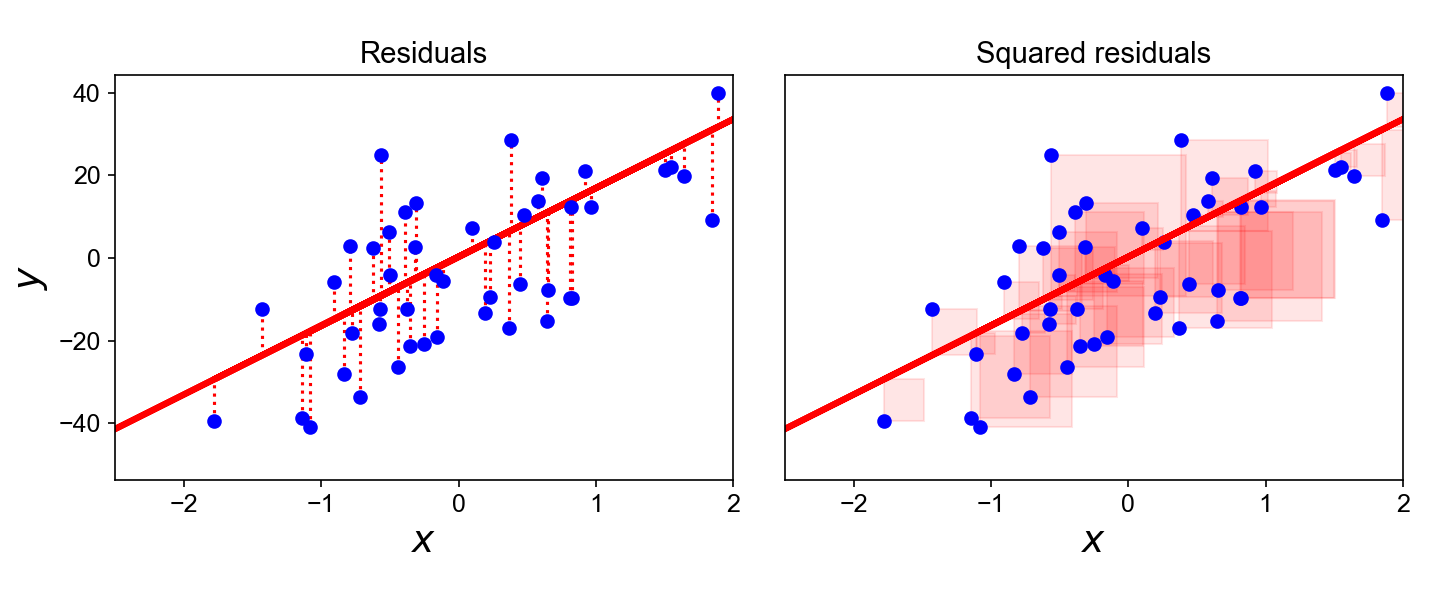
The image below illustrates this concept. The blue dots are the data points, the red line is the fitted model $\hat{y}=X\hat{\beta }$. The dotted red lines are the residuals $e_n$, and the goal of OLS is to adjust the slope and intercept of the red line to make the total area of the red squares (the squared residuals) as small as possible.

The Geometric Viewpoint

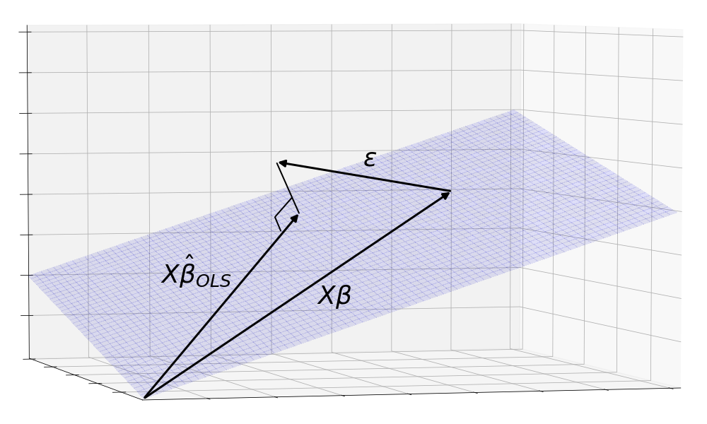
There's a beautiful geometric interpretation of this process that directly leverages our work on vector projections. The vector of predictions, $\hat{y}=X\hat{\beta }$, is a linear combination of the columns of $X$. This means $\hat{y}$ must lie in the column space of $X$, denoted $\text{Col}(X)$.

The OLS problem is thus equivalent to finding the vector $\hat{y}$ in the subspace $\text{Col}(X)$ that is closest to the observed vector $y$. As we know from our lesson on projections, the vector in the subspace closest to $y$ is its orthogonal projection. This means the residual vector, $e=y-\hat{y}$, must be orthogonal to the entire column space of $X$.

The Derivation: Applying Matrix Calculus

We have our objective function: $J(\hat{\beta })=(y-X\hat{\beta }{)}^T(y-X\hat{\beta })$. From calculus, we know that to find the minimum of a function, we take its derivative, set it to zero, and solve. Here, our variable $\hat{\beta }$ is a vector, so we need to compute the gradient.

This leads to our Socratic question for today:

We need to find ${\nabla }_{\hat{\beta }}J(\hat{\beta })$. Let's first expand the objective function. What does $(y-X\hat{\beta }{)}^T(y-X\hat{\beta })$ become when you apply the transpose rules?

Think about how you would expand $(a-b{)}^2$. The matrix equivalent is $(A-B{)}^T(A-B)$ which expands to $A^{T}A-A^{T}B-B^{T}A+B^{T}B$.

Let's apply this:

$$\begin{array}{rl}J(\hat{\beta })& =(y^T-(X\hat{\beta }{)}^T)(y-X\hat{\beta })\\ & =(y^T-{\hat{\beta }}^T{X}^T)(y-X\hat{\beta })\\ & =y^{T}y-y^{T}X\hat{\beta }-{\hat{\beta }}^T{X}^{T}y+{\hat{\beta }}^T{X}^{T}X\hat{\beta }\end{array}$$

Notice that $y^{T}X\hat{\beta }$ is a scalar (a $1\times N\cdot N\times P\cdot P\times 1\to 1\times 1$). The transpose of a scalar is just itself. So, $(y^{T}X\hat{\beta }{)}^T={\hat{\beta }}^T{X}^{T}y$. This means the two middle terms are identical. Our objective function simplifies to:

$$J(\hat{\beta })=y^{T}y-2{\hat{\beta }}^T{X}^{T}y+{\hat{\beta }}^T{X}^{T}X\hat{\beta }$$

Now, we need to differentiate this expression with respect to the vector $\hat{\beta }$. This requires a couple of key matrix calculus identities. The following video provides excellent intuition by building up from simple scalar derivatives to the vector and matrix forms we need.

From the video and our calculus background, we have the two main results we need:

1. ${\nabla }_x(a^{T}x)=a$
2. ${\nabla }_x(x^{T}Ax)=2Ax$ (for a symmetric matrix $A$)

Let's apply these to our objective function term by term:

$${\nabla }_{\hat{\beta }}J(\hat{\beta })={\nabla }_{\hat{\beta }}(y^{T}y)-{\nabla }_{\hat{\beta }}(2{\hat{\beta }}^T{X}^{T}y)+{\nabla }_{\hat{\beta }}({\hat{\beta }}^T{X}^{T}X\hat{\beta })$$

• Term 1: $y^{T}y$ is a scalar constant with respect to $\hat{\beta }$, so its derivative is $0$.
• Term 2: Using ${\nabla }_x(a^{T}x)=a$, we treat $\hat{\beta }$ as $x$ and $2X^{T}y$ as $a$. The derivative is $2X^{T}y$.
• Term 3: Using ${\nabla }_x(x^{T}Ax)=2Ax$, we treat $\hat{\beta }$ as $x$ and $X^{T}X$ as $A$. Note that $X^{T}X$ is always symmetric, so the rule applies. The derivative is $2(X^{T}X)\hat{\beta }$.

Combining these, we get the gradient:

$${\nabla }_{\hat{\beta }}J(\hat{\beta })=-2X^{T}y+2(X^{T}X)\hat{\beta }$$

To find the minimum, we set the gradient to zero:

$$-2X^{T}y+2(X^{T}X)\hat{\beta }=0$$ $$2(X^{T}X)\hat{\beta }=2X^{T}y$$

This gives us the famous Normal Equations:

$$(X^{T}X)\hat{\beta }=X^{T}y$$

This equation is fundamental. It arises directly from the condition that the residual vector must be orthogonal to the column space of $X$, i.e., $X^T(y-X\hat{\beta })=0$, which simplifies to the same result.

To get the final solution for $\hat{\beta }$, we just need to solve this linear system. If the matrix $(X^{T}X)$ is invertible (which is true if the columns of $X$ are linearly independent), we can pre-multiply both sides by its inverse:

$$(X^{T}X{)}^{-1}(X^{T}X)\hat{\beta }=(X^{T}X{)}^{-1}{X}^{T}y$$ $$I\hat{\beta }=(X^{T}X{)}^{-1}{X}^{T}y$$

And there we have it, the closed-form solution for the Ordinary Least Squares estimator:

$${\hat{\beta }}_{\text{OLS}}=(X^{T}X{)}^{-1}{X}^{T}y$$

For a comprehensive walkthrough of this entire derivation, I highly recommend the following reading and video.

Conclusion

In this lesson, we have derived the closed-form solution for Ordinary Least Squares from first principles. This is a classic result in statistics and machine learning and a perfect illustration of an optimization problem that can be solved analytically. By defining a cost function—the sum of squared residuals—we were able to use matrix calculus to find the exact parameters that minimize it.

Key Takeaways:

• Linear regression can be expressed compactly using matrix notation as $y=X\beta +ϵ$.
• The OLS objective is to minimize the sum of squared residuals, $J(\hat{\beta })=(y-X\hat{\beta }{)}^T(y-X\hat{\beta })$.
• Geometrically, OLS finds the orthogonal projection of the observed data vector $y$ onto the subspace spanned by the feature matrix $X$.
• By setting the gradient of the objective function to zero, we derive the Normal Equations: $(X^{T}X)\hat{\beta }=X^{T}y$.
• Solving the Normal Equations gives the closed-form OLS solution: $\hat{\beta }=(X^{T}X{)}^{-1}{X}^{T}y$.

Preview of the Next Lesson:

The ability to find a direct, analytical solution like this is powerful, but rare. The calculation involves inverting the $(X^{T}X)$ matrix, an operation that is computationally expensive and numerically unstable for very large or ill-conditioned matrices. More importantly, for the vast majority of models in deep learning—with their nested non-linear functions and millions of parameters—no such closed-form solution exists. We simply cannot "solve for $\beta$" by inverting a matrix.

This limitation is precisely what motivates the need for iterative optimization. In our next lesson, we will explore the fundamental trade-offs between closed-form and iterative methods and derive the workhorse algorithm of all of deep learning: gradient descent.