Cross-Entropy and KL Divergence: Measuring Distribution Differences

Recommended resources

The freely available resources this lesson will direct you to.

Introduction

In our previous lesson, we established a crucial link between statistics and machine learning: minimizing the binary cross-entropy (BCE) loss function is mathematically equivalent to performing Maximum Likelihood Estimation (MLE) on a model that assumes a Bernoulli-distributed output. This provided a principled, probabilistic foundation for a core component of deep learning.

Today, we will generalize this understanding by stepping back and examining cross-entropy and the related Kullback-Leibler (KL) divergence from the perspective of information theory. This will provide you with a deeper intuition for why these functions are such effective measures for comparing probability distributions. By the end of this lesson, you will be able to define and interpret both cross-entropy and KL divergence, understand their fundamental relationship, and see why they are the preferred objective functions for training classification models.

From Information to Entropy

At the heart of information theory is the idea of quantifying "information" or "surprise." An event that is very unlikely carries a lot of information when it occurs, while a very likely event carries little. Claude Shannon formalized this by defining the information content of an event $x$ with probability $p (x)$ as:

I (x) = - lo g_{2} p (x) (in bits)

The negative sign makes the result positive, and the logarithm ensures that information from independent events is additive.

If we have a full probability distribution, we can ask: what is the average amount of information we get from one sample drawn from this distribution? This average is called Shannon Entropy, denoted $H (p)$ . It is the expectation of the information content over the distribution $p$ :

H (p) = E_{x \sim p} [I (x)] = E_{x \sim p} [- lo g_{2} p (x)] = - i \sum p (x_{i}) lo g_{2} p (x_{i})

Entropy can be interpreted as a measure of the uncertainty inherent in a distribution. A distribution with high entropy is highly unpredictable (like a fair coin flip), while one with low entropy is predictable (like a biased coin that almost always lands heads). From a coding perspective, entropy represents the theoretical minimum average number of bits required to encode messages drawn from distribution $p$ .

The following video provides an excellent intuitive introduction to entropy, building up the concept with clear examples.

A Short Introduction to Entropy, Cross-Entropy and KL-Divergence

This video from Aurélien Géron, author of "Hands-On Machine Learning," offers a short, clear introduction to these information-theoretic concepts.

Watch the segment on entropy, from the beginning to the start of the cross-entropy section. Pay close attention to how the amount of information is related to the reduction in uncertainty and how entropy is calculated as the weighted average of the information of all possible outcomes.

Cross-Entropy: The Cost of a Suboptimal Code

Entropy tells us the optimal average code length for a distribution $p$ . But what if we design a code based on an incorrect distribution, let's call it $q$ , and use it to encode events that are actually drawn from the true distribution $p$ ? The resulting average code length is called the cross-entropy, $H (p, q)$ .

The formula is very similar to entropy, but the logarithm uses the probabilities from our assumed distribution $q$ , while the expectation is still taken over the true distribution $p$ :

H (p, q) = E_{x \sim p} [- lo g_{2} q (x)] = - i \sum p (x_{i}) lo g_{2} q (x_{i})

In machine learning, $p$ represents the "ground truth" distribution (e.g., the one-hot encoded true label), and $q$ represents the predicted probability distribution from our model. Cross-entropy, therefore, measures the average number of bits needed to encode the true outcomes if we use our model's predictions to build the code. The closer our predictions $q$ are to the truth $p$ , the lower the cross-entropy will be.

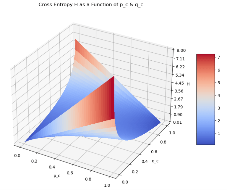
This plot visualizes binary cross-entropy, $H(p, q) = -p_c \log q_c - (1-p_c) \log (1-q_c)$, as a function of the true probability $p_c$ and the predicted probability $q_c$ for a single class. The loss is minimized (H=0) along the diagonal line where $p_c = q_c$, meaning the prediction matches the truth. The loss grows infinitely as the prediction $q_c$ approaches the opposite of the truth (e.g., predicting 0 when the truth is 1).

Let's continue with the video from Aurélien Géron, which now explains cross-entropy using this coding analogy.

A Short Introduction to Entropy, Cross-Entropy and KL-Divergence

This part of the video explains how using a code optimized for the wrong distribution leads to a higher average message length, which is precisely what cross-entropy measures.

Please watch the segment from the start of the cross-entropy section up to the introduction of KL-Divergence.

KL Divergence: The "Penalty" for Being Wrong

We now have two quantities:

Entropy $H (p)$ : The ideal average code length for distribution $p$ .
Cross-Entropy $H (p, q)$ : The average code length we actually get when using a code based on $q$ for events from $p$ .

It's a fundamental result of information theory (Gibbs' inequality) that $H (p, q) \geq H (p)$ , with equality only if $p = q$ . This means our suboptimal code is always less efficient than or equal to the optimal one.

The difference between these two quantities—the extra bits we need on average due to using the wrong distribution $q$ —is called the Kullback-Leibler (KL) Divergence, also known as relative entropy.

D_{K L} (p ∣∣ q) = H (p, q) - H (p)

KL Divergence quantifies the information "lost" when we use $q$ to approximate $p$ . It's a measure of how different the two distributions are.

Let's expand the formula:

D_{K L} (p ∣∣ q) = (- i \sum p (x_{i}) lo g_{2} q (x_{i})) - (- i \sum p (x_{i}) lo g_{2} p (x_{i})) = i \sum p (x_{i}) lo g_{2} p (x_{i}) - i \sum p (x_{i}) lo g_{2} q (x_{i}) = i \sum p (x_{i}) (lo g_{2} p (x_{i}) - lo g_{2} q (x_{i})) = i \sum p (x_{i}) lo g_{2} \frac{p ( x _{i} )}{q ( x _{i} )}

For continuous distributions, the sum is replaced by an integral.

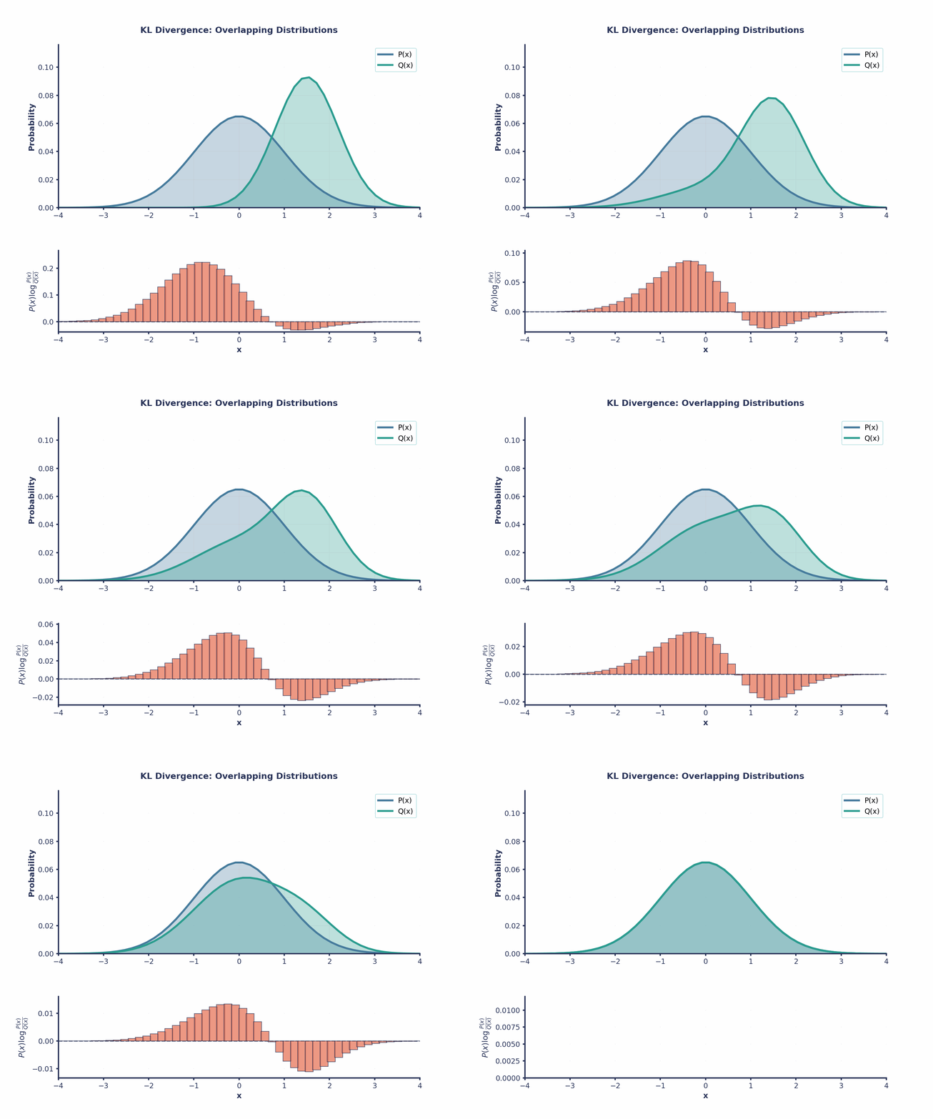
This visualization shows two distributions, P(x) and Q(x). The bottom plot shows the value of the term $P(x) \log \frac{P(x)}{Q(x)}$ at each point x. The total KL divergence is the sum (or integral) of these values. Where P(x) is high and Q(x) is low, the ratio is large, contributing significantly to the divergence. Where the distributions are similar, the ratio is close to 1, $\log(1)=0$, and the contribution is minimal.

Now, let's watch the final conceptual piece of the video, connecting these ideas.

A Short Introduction to Entropy, Cross-Entropy and KL-Divergence

This segment formally defines KL-Divergence as the difference between cross-entropy and entropy.

Watch from the introduction of KL-Divergence to the start of the machine learning section.

Properties of KL Divergence

KL Divergence has two crucial properties:

Non-negativity: $D_{K L} (p ∣∣ q) \geq 0$ , with $D_{K L} (p ∣∣ q) = 0$ if and only if $p = q$ .
Asymmetry: In general, $D_{K L} (p ∣∣ q) \neq = D_{K L} (q ∣∣ p)$ .

This asymmetry is important. It means KL divergence is not a true mathematical distance metric (like Euclidean distance). It's a divergence. The order matters: $D_{K L} (p ∣∣ q)$ measures the information lost when approximating the true distribution $p$ with $q$ , which is different from approximating $q$ with $p$ .

An Alternative View: KL Divergence and Likelihood Ratios

Given your background with Maximum Likelihood Estimation, there's another powerful way to interpret KL divergence. It can be derived by thinking about how distinguishable two distributions are based on the data they generate.

Imagine we have two coins, one with a true probability distribution $p$ and another with distribution $q$ . We flip the first coin many times and get a sequence of observations. A natural way to measure the difference between $p$ and $q$ is to ask: "How much more likely is this sequence of observations under the true distribution $p$ compared to the other distribution $q$ ?"

This leads to considering the ratio of likelihoods. The following video masterfully shows how the KL divergence formula naturally emerges from formalizing this idea of a normalized log-likelihood ratio. This provides a direct bridge from the statistical ideas of MLE to the information-theoretic concept of KL divergence.

Intuitively Understanding the KL Divergence

This video by Adian Liusie offers a unique and intuitive derivation of KL Divergence, starting from the idea of comparing the likelihood of observations under two different distributions.

Please watch from the coin example. Follow the derivation that starts with a simple likelihood ratio and, through logarithmic manipulation and taking the limit, arrives at the exact formula for KL divergence. This beautifully connects what we learned about likelihood in the previous lessons to today's topic.

From Theory to Practice: Cross-Entropy vs. KL Divergence in ML

We've established the relationship:

Cross-Entropy H (p, q) = KL Divergence D_{K L} (p ∣∣ q) + Entropy H (p)

Our goal in training a model is to make our predicted distribution $q_{θ}$ (where $θ$ are the model parameters) as close as possible to the true data distribution $p$ . This is equivalent to minimizing $D_{K L} (p ∣∣ q_{θ})$ .

So, if our goal is to minimize KL divergence, why are machine learning loss functions almost always cross-entropy?

In a typical supervised learning problem, the true distribution $p$ is fixed—it's determined by the training dataset. Therefore, the entropy of the true distribution, $H (p)$ , is a constant with respect to our model parameters $θ$ . When we are looking for the parameters $θ$ that minimize a function, we can ignore any constant terms.

ar g θ min H (p, q_{θ}) = ar g θ min [D_{K L} (p ∣∣ q_{θ}) + H (p)] = ar g θ min D_{K L} (p ∣∣ q_{θ})

Minimizing cross-entropy with respect to $θ$ is equivalent to minimizing KL divergence. We use cross-entropy in practice because it's simpler to calculate—we only need $p (x)$ and $q_{θ} (x)$ , and we don't need to compute the $H (p)$ term.

The following resource provides the formal definitions and explicitly derives this equivalence.

Cross Entropy, KL Divergence, and Maximum Likelihood ...

This blog post by Lei Mao provides concise mathematical definitions and clearly shows the relationships between these concepts.

First, review the definitions in the sections "Cross Entropy" and "Kullback-Leibler Divergence" to solidify the formulas. Note that the author uses natural log (\ln) which is standard in ML, whereas information theory often uses base-2 log (\log_2). This is just a constant factor difference (\ln x = \ln 2 \cdot \log_2 x) and doesn't affect optimization. Next, read the derivation in the section "Cross Entropy and KL Divergence", which shows how D_{KL}(p||q) is derived from H(p,q) and H(p). Finally, study the section "Optimization Using Cross Entropy or KL Divergence". This is the key takeaway, as it formally shows why minimizing cross-entropy is equivalent to minimizing KL divergence during model training.

Conclusion

In this lesson, we ventured into information theory to build a first-principles understanding of the objective functions that drive modern classification models. We saw that these concepts are not arbitrary but are grounded in the logic of efficient coding and information transfer.

Key Takeaways:

Entropy $H (p)$ : A measure of the inherent uncertainty in a probability distribution $p$ . It represents the minimum average bits needed to encode an event from $p$ .
Cross-Entropy $H (p, q)$ : Measures the average bits needed to encode an event from a true distribution $p$ using a code designed for a predicted distribution $q$ . It serves as a powerful loss function in machine learning.
KL Divergence $D_{K L} (p ∣∣ q)$ : The "penalty" or extra bits required due to using $q$ to approximate $p$ . It quantifies the difference between two distributions and is defined as $H (p, q) - H (p)$ .
Optimization Equivalence: In training, minimizing the cross-entropy loss $H (p, q_{θ})$ is equivalent to minimizing the KL divergence $D_{K L} (p ∣∣ q_{θ})$ because the true data entropy $H (p)$ is a constant.

Preview of the Next Module:

We now have a deep understanding of what we are optimizing—objective functions like Negative Log-Likelihood and Cross-Entropy that measure the "distance" between our model's predictions and reality. The next fundamental question is how do we perform this optimization?

In the next module, we will begin our deep dive into Numerical Optimization. We will first examine a classical model, Ordinary Least Squares, which admits an elegant, direct closed-form solution. We will then see why such solutions are impossible for complex deep learning models, motivating the need for iterative optimization methods, starting with the algorithm that powers all of deep learning: gradient descent.