Vectorized Numerical Operations with NumPy Arrays

Hello! Last time, you moved reusable Python functions into a package. Today you’ll add numerical work to that same project. NumPy arrays let you apply arithmetic to many values at once, then summarize the results without writing a loop for each calculation. That pattern will be useful when you begin working with datasets and model outputs. Allow about 40 minutes, including time to run the examples.

From individual values to array operations

Suppose you have three measurements and need to increase each by two. With a Python list, you could loop over its elements. A NumPy array lets you express the calculation for the whole collection:

import numpy as np

measurements = np.array([10, 20, 30])
print(measurements + 2)  # [12 22 32]

This is vectorized arithmetic: you specify an operation on an array, and NumPy handles the element-by-element work. It does not mean NumPy necessarily runs the calculation on multiple CPU cores. The immediate benefits are that the code describes the intended calculation directly and avoids a Python-level loop for each element.

Start with the array-creation portion of Python NumPy Tutorial for Beginners from freeCodeCamp.org. Concentrate on the distinction between a one-dimensional collection and a two-dimensional array of rows and columns; you do not need to memorize every array-creation function shown.

An array’s .shape reports its size along each axis. For a two-dimensional array, that means (number_of_rows, number_of_columns). Its .dtype describes the type of values stored. Check both when a calculation produces an unexpected result:

readings = np.array([[10, 20, 30],
                     [12, 22, 32]])

print(readings.shape)  # (2, 3)
print(readings.dtype)  # typically an integer dtype

NumPy arrays and Python lists do not interpret every operator the same way. Adding two lists joins them; adding two same-shaped numeric arrays adds corresponding elements. Multiplication with * is elementwise too—it is not matrix multiplication.

first = np.array([10, 20, 30])
second = np.array([1, 2, 3])

print(first + second)  # [11 22 33]
print(first * second)  # [10 40 90]
print(first / 10)      # [1. 2. 3.]
print(first ** 2)      # [100 400 900]

Each result above is a new array; first remains unchanged. NumPy also supplies functions that act across an array, such as np.sqrt(np.array([4, 9, 16])), which produces [2. 3. 4.].

Return to the same tutorial for its demonstrations of arithmetic and summary calculations. You can skip the intervening linear-algebra section: matrix multiplication is a different operation from the elementwise arithmetic we need here.

Broadcasting: when shapes differ usefully

Arrays do not always need identical shapes. NumPy can broadcast a smaller input across a larger one when their dimensions are compatible. You have already used the simplest case: measurements + 2 applies one scalar value to every element.

Read the Broadcasting section of NumPy’s Absolute Basics for Beginners. Its distance-conversion example introduces the idea without requiring new syntax.

The supplied broadcasting diagram shows a more useful case. A four-row, one-column array combines with a three-element array to produce four rows and three columns:

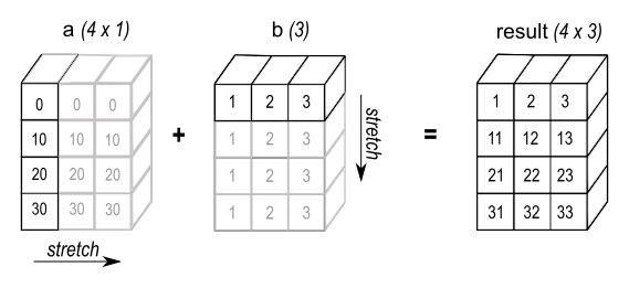
To predict whether broadcasting will work, compare shapes from their rightmost dimensions. Each pair must match, or one of the two sizes must be 1. A missing leading dimension is treated as 1 for this comparison. Thus (4, 1) and (3,) can produce (4, 3): the second shape behaves like (1, 3).

This matters when applying one adjustment per column of a dataset:

readings = np.array([[10, 20, 30],
                     [12, 22, 32]])
adjustments = np.array([1, -2, 3])

print(readings + adjustments)
# [[11 18 33]
#  [13 20 35]]

The shapes are (2, 3) and (3,), so the same three adjustments apply to each row. If adjustments instead had two elements, its shape (2,) would conflict with the readings’ rightmost dimension of 3, and NumPy would raise a ValueError. Before relying on broadcasting, check that the resulting shape—and the direction in which values repeat—matches your intent.

Reduce many values to a useful summary

Elementwise operations retain an array of results. An aggregation combines values into a summary. For example, readings.sum() adds every value, while readings.mean() calculates one average for the entire array.

For a two-dimensional array, axis specifies which dimension is reduced:

readings = np.array([[10, 20, 30],
                     [12, 22, 32]])

print(readings.mean(axis=0))  # [11. 21. 31.]
print(readings.mean(axis=1))  # [20. 22.]

With axis=0, NumPy reduces across rows, leaving one mean per column. With axis=1, it reduces across columns, leaving one mean per row. A useful check is the output length: a column summary of a (2, 3) array has three values; a row summary has two. The same axis choice works with methods such as .sum(), .min(), and .max().

You can combine broadcasting, elementwise arithmetic, and aggregation without manually processing each reading. If every column has its own adjustment, first add the adjustments to the whole array; then take mean(axis=0) to get one adjusted average per column.

Put the calculation in your project

Activate the .venv you created earlier, using the command for your system from the first lesson. From the outer ai-workflows directory, install NumPy and update the environment’s pinned package list:

python -m pip install numpy
python -m pip freeze > requirements.txt

For this small environment, pip freeze records the exact versions installed, including any dependencies. Now create ai_workflows/numeric_utils.py beside text_utils.py:

import numpy as np


def calibrate_and_average(readings, adjustments):
    """Adjust each column, then return the adjusted array and column means."""
    values = np.asarray(readings, dtype=float)
    offsets = np.asarray(adjustments, dtype=float)

    adjusted = values + offsets
    column_means = adjusted.mean(axis=0)
    return adjusted, column_means

np.asarray accepts either a suitable existing array or a sequence such as a list. Here, dtype=float makes the intended numerical type explicit. This function expects two-dimensional readings and a one-dimensional adjustment with one value per column; the addition uses broadcasting, and the mean reduces across rows.

Create run_numeric_demo.py in the outer project directory:

import numpy as np

from ai_workflows.numeric_utils import calibrate_and_average


def main():
    readings = np.array([
        [10, 20, 30],
        [12, 22, 32],
        [14, 24, 34],
        [16, 26, 36],
    ])
    adjustments = np.array([1, -2, 3])

    adjusted, column_means = calibrate_and_average(
        readings, adjustments
    )

    print("Input shape:", readings.shape)
    print("Adjusted readings:\n", adjusted)
    print("Column means:", column_means)


if __name__ == "__main__":
    main()

Run python run_numeric_demo.py from ai-workflows. The adjusted rows should be [11, 18, 33], [13, 20, 35], [15, 22, 37], and [17, 24, 39]; the column means should be [14. 21. 36.]. You have performed calculations across twelve readings without writing a loop over those readings.

Takeaways

NumPy arrays apply arithmetic elementwise; broadcasting lets compatible shapes share values across dimensions; and aggregations such as .mean(axis=0) turn a whole array into the summary you need. Checking .shape is often the fastest way to understand—or debug—each step.

Next, you’ll work with pandas DataFrames, where numerical columns sit alongside row labels and other tabular information. The idea of operating on a whole collection rather than processing one value at a time will carry forward.