Strong vs. Weak Scaling for Distributed Systems

Introduction

In our last lesson, we focused on analyzing profiler traces to pinpoint performance limiters within a distributed system at a fixed scale. We learned to identify the tell-tale signs of CPU bottlenecks, data movement overhead, and expensive compute kernels. This analysis tells us why a single step takes as long as it does.

Today, we move from the "what" to the "how well." This lesson addresses the learning outcome: Explain how to reason about strong vs. weak scaling to evaluate the efficiency of a distributed system. We will explore the two fundamental models for evaluating how a system's performance changes as we add more resources, like GPUs. This is crucial for designing and justifying large-scale AI systems. You will learn to answer two key questions:

1. How much faster can I solve my fixed-size problem by adding more GPUs?
2. How much more work can I do in the same amount of time by adding more GPUs?

By the end of this lesson, you will understand the theoretical laws that govern parallel speedup and be able to apply them to predict and evaluate the efficiency of distributed training systems.

Framing Scalability: From Algorithms to Systems

Given your background, you are certainly familiar with algorithmic scalability, typically expressed using Big-O notation. This describes how an algorithm's runtime or memory usage grows with the size of its input $n$ on a single machine.

In distributed systems, we are concerned with a different kind of scalability: how the system's performance changes as we add more processing units (e.g., GPUs). This is often called horizontal scaling—adding more machines to share the load. This is distinct from vertical scaling, which means using a single, more powerful machine. Our focus in large-scale AI is almost exclusively on horizontal scaling.

Strong and weak scaling are the two primary frameworks for measuring the effectiveness of horizontal scaling.

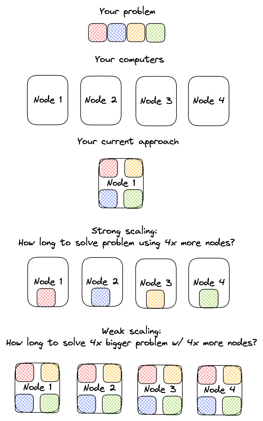
Let's start with a simple visual that cleanly separates these two concepts.

Strong Scaling: The Pursuit of Speed (Amdahl's Law)

Strong scaling addresses the first question: how much faster can we solve a fixed-size problem by adding more resources? The goal is to minimize the time-to-solution.

The theoretical limit of strong scaling is described by Amdahl's Law. The law states that the speedup of a program using multiple processors is limited by the fraction of the program that must be executed sequentially.

To formalize this, please watch the following video segments. They introduce Amdahl's Law, its formula, and the important concept of efficiency.

Connecting to Profiling

Amdahl's Law provides the theoretical lens for interpreting the bottlenecks we identified in the previous lesson. The serial fraction ($1-f$) in Amdahl's equation is precisely the overhead that is not parallelized across GPUs. In a profiler trace, this corresponds to:

• Data loading and preprocessing on the CPU.
• Idle time caused by CPU-GPU synchronization points (like loss.item()).
• Final reduction or aggregation steps that run on a single node.
• Inter-GPU communication overhead (e.g., AllReduce) which, while parallel, may not scale perfectly and acts as a serializing bottleneck.

This article provides an excellent summary of Amdahl's Law in the context of GPU computing.

Weak Scaling: The Pursuit of Capacity (Gustafson's Law)

Weak scaling addresses the second question: how much bigger a problem can we solve by adding more resources, assuming we keep the total run time constant? Here, the goal is to increase throughput or problem size.

This perspective is captured by Gustafson's Law. It argues that as we get more processors, we tend to tackle larger problems. Gustafson's insight was that the parallel part of the workload scales with the number of processors, while the serial part often remains fixed.

Let's return to the video to understand the formulation of Gustafson's Law.

In the context of deep learning, weak scaling corresponds to increasing the global batch size as you add more GPUs. If you go from 1 to 8 GPUs and increase your batch size from 256 to 2048, you are performing weak scaling. Your goal is often to keep the time per epoch roughly constant while processing 8x more data, thus maintaining high efficiency.

This article nicely frames Gustafson's law for GPU-centric workloads.

Synthesis: Two Laws, One Reality

Amdahl's and Gustafson's laws are not contradictory; they are different perspectives for different goals.

• Amdahl (Strong Scaling): Your problem is fixed. You want it done faster. You are limited by serial overhead.
• Gustafson (Weak Scaling): Your time is fixed. You want to do more work. You can maintain high efficiency if the workload scales.

In practice, most large-scale training scenarios are a mix of both. You want to reduce the time per step (strong scaling), but you also increase the batch size to effectively use more GPUs (weak scaling).

This article provides a superb real-world example applying both concepts to multi-GPU training.

A Deeper Mathematical Connection

Given your theoretical background, you might appreciate that these two laws are more than just different perspectives—they are mathematically two sides of the same coin. One can be derived from the other by reformulating the assumptions. The key is recognizing that the absolute time spent on the sequential part of the program is the constant.

The following paper provides a concise and elegant formal derivation.

This derivation clarifies that the "pessimism" of Amdahl and the "optimism" of Gustafson arise simply from how you define the problem context: one fixes the total work, the other fixes the total time.

Conclusion

Today we explored the two essential frameworks for reasoning about the performance of distributed systems. Understanding both strong and weak scaling is fundamental to designing, evaluating, and justifying large-scale AI infrastructure.

Key Takeaways:

• Strong Scaling (Amdahl's Law) measures how much faster you can solve a fixed-size problem. It's limited by the serial fraction of your workload, leading to diminishing returns as you add processors. Your goal is to minimize run-time.
• Weak Scaling (Gustafson's Law) measures how much larger a problem you can solve in a fixed amount of time. It offers a more optimistic view, suggesting that efficiency can remain high if the problem size scales with the number of processors. Your goal is to maximize throughput.
• Metrics: Speedup ($S=T_1/T_N$) and Efficiency ($E=S/N$) are the key metrics for evaluating both types of scaling. Ideal weak scaling maintains a constant efficiency close to 100%. Ideal strong scaling achieves the maximum speedup possible.
• Practical Relevance: In distributed training, Amdahl's law explains why communication and other overheads cap your speedup for a fixed batch size. Gustafson's law explains why increasing the global batch size is a common and effective strategy to maintain high GPU utilization as you scale out.

Preview of the Next Lesson:

We've established that communication overhead is a critical component of the "serial fraction" that limits strong scaling. In our next lesson, "Describe how topology-aware task placement can optimize collective communication performance," we will investigate a concrete strategy to attack this bottleneck. We'll explore how the physical layout of GPUs and the network connections between them (the "topology") can be exploited to reduce communication costs and improve scaling efficiency.