Real Estate Correlation Calculation

Hello! Welcome back to our final module on Real Estate Portfolio Management and Optimization.

In our last lesson, we learned how to quantify portfolio concentration using the Herfindahl-Hirschman Index (HHI). This gave us a powerful tool to measure how much our portfolio's value is packed into specific geographic markets or property types. We now understand how to measure our "eggs in one basket" risk.

Today, we'll add the second crucial piece to our portfolio risk analysis. It's not enough to know how many baskets we have; we must also understand if picking up one basket causes all the others to jiggle in the same way. This is the concept of correlation. Our learning outcome for this lesson is to calculate the correlation of returns between different real estate assets in a portfolio. This metric is the engine of diversification and a fundamental input for portfolio optimization.

1. Understanding Correlation of Returns

Correlation is a statistical measure of how two variables move in relation to each other. The correlation coefficient, typically denoted as $r$ (rho), ranges from -1 to +1:

• +1 (Perfect Positive Correlation): The assets' returns move in perfect lockstep. If one goes up 5%, the other goes up 5%.
• 0 (No Linear Correlation): The returns of the assets are unrelated. The movement of one provides no information about the movement of the other.
• -1 (Perfect Negative Correlation): The assets' returns move in perfect opposition. If one goes up 5%, the other goes down 5%.

In portfolio management, our goal is to combine assets with low, or ideally negative, correlation. This is the mathematical heart of diversification: when one asset performs poorly, the others are likely to be performing differently (either neutrally or well), smoothing out the overall portfolio return.

Why "Returns" and Not "Prices"?

This is a critical distinction. It might seem intuitive to correlate property prices, but this is a common statistical trap. Most asset prices, including real estate, tend to trend upwards over long periods due to inflation and economic growth. Correlating two variables that are both independently trending upwards will almost always produce a high positive correlation, even if their underlying drivers are completely unrelated. This is called spurious correlation.

To get a meaningful measure of the relationship, we must analyze the correlation of their returns (i.e., the percentage changes in value over a period). To see a clear explanation of this concept, please watch the following short video.

2. Calculating the Correlation Coefficient

The most common correlation coefficient is the Pearson correlation coefficient. Its formula looks complex, but the intuition is straightforward: it measures the extent to which two variables vary together from their respective means.

For two series of returns, $R_i$ and $R_j$, the correlation coefficient ${\rho }_{ij}$ is calculated as the covariance between them divided by the product of their standard deviations.

Where:

• $\text{Cov}(R_i,R_j)$ is the covariance between the returns of asset $i$ and asset $j$.
• ${\sigma }_i$ and ${\sigma }_j$ are the standard deviations of the returns for asset $i$ and asset $j$, respectively.

You can see this formula presented in the context of portfolio theory in the following resource.

While understanding the formula is good, as a software engineer, you'll be glad to know that we can rely on Python libraries to handle these calculations for us with high efficiency.

3. Practical Calculation with Python and Spanish Data

Let's put this into practice. For real estate, we don't have daily price ticks like we do for stocks. We typically work with annual, semi-annual, or quarterly returns data, which can be derived from valuation appraisals or market indices.

Let's use the chart below, which shows the evolution of prime yields in Spain for different property types, to create a hypothetical returns dataset. Remember that yield and price are inversely related: a falling yield implies rising prices (positive capital return), and a rising yield implies falling prices (negative capital return).

Let's imagine we have a portfolio with three assets and we've calculated their annual capital returns for the past 5 years. We can model this data in Python using the pandas library.

import pandas as pd
import numpy as np

# Hypothetical annual capital returns (%) for three assets in our portfolio
# Inspired by the trends in the yield chart above.
data = {
    'Madrid_Office':    [3.0, 3.5, 4.0, 1.0, -1.0], # Stable, then a downturn
    'Barcelona_Apt':    [4.0, 4.5, 5.0, 2.5,  0.5], # Similar to office but slightly more resilient
    'Valencia_Logistic':[6.0, 7.0, 8.0, 9.0,  5.0]  # Strong growth trend (like falling logistics yields)
}

# Create a DataFrame
# The index represents the year (e.g., 2019, 2020, 2021, 2022, 2023)
returns_df = pd.DataFrame(data)

print("Annual Returns (%):")
print(returns_df)

Now that we have our data in a DataFrame, calculating the correlation matrix is incredibly simple with the .corr() method.

# Calculate the correlation matrix
correlation_matrix = returns_df.corr()

print("\nCorrelation Matrix:")
print(correlation_matrix)

Output of the Code:

Annual Returns (%):
   Madrid_Office  Barcelona_Apt  Valencia_Logistic
0            3.0            4.0                6.0
1            3.5            4.5                7.0
2            4.0            5.0                8.0
3            1.0            2.5                9.0
4            -1.0           0.5                5.0

Correlation Matrix:
                   Madrid_Office  Barcelona_Apt  Valencia_Logistic
Madrid_Office           1.000000       0.989725           0.457882
Barcelona_Apt           0.989725       1.000000           0.604618
Valencia_Logistic       0.457882       0.604618           1.000000

Interpreting the Correlation Matrix

This matrix is the final product. Here's how to read it:

• The diagonal is always 1.0, as an asset is perfectly correlated with itself.
• The matrix is symmetrical (the correlation of A to B is the same as B to A).
• Madrid Office vs. Barcelona Apt ($\approx 0.99$): This extremely high correlation suggests these two assets move in near-perfect lockstep. Adding the Barcelona apartment to a portfolio that already holds the Madrid office provides very little diversification benefit. Their risk factors are likely very similar (e.g., both are prime offices in major Spanish cities, sensitive to the same macroeconomic business cycles).
• Madrid Office vs. Valencia Logistics ($\approx 0.46$): This is a moderately positive correlation. They tend to move in the same direction, but not tightly. This indicates that the logistics asset provides a good diversification benefit to the office asset. Its returns are driven by different factors (e.g., e-commerce, supply chain dynamics) than prime office space.
• Barcelona Apt vs. Valencia Logistics ($\approx 0.60$): A higher correlation than with the office, but still providing meaningful diversification.

For an in-depth guide on the different ways to calculate correlation in Python (using NumPy, SciPy, and pandas) and how to visualize the results, the following article is an excellent resource for your background.

4. Visualizing the Correlation Matrix

As the Real Python article explains, a table of numbers becomes hard to interpret with many assets. The standard professional practice is to visualize the correlation matrix as a heatmap.

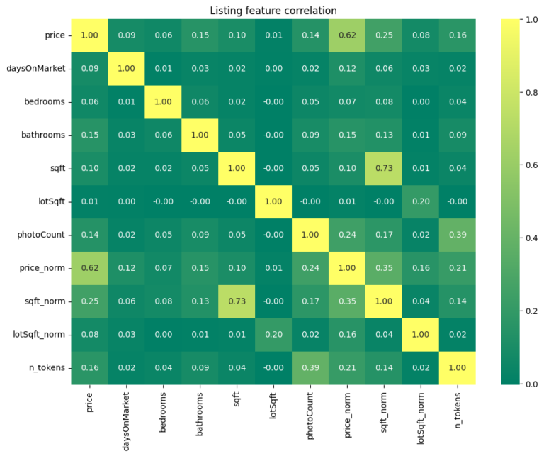
Using the code from the recommended article, you could generate a similar heatmap for our example, making it immediately obvious that the two office assets are highly correlated while the logistics asset stands apart.

Conclusion

You have now mastered the second fundamental component of portfolio risk analysis. By calculating the correlation of returns, you can move beyond simply owning different assets to strategically combining assets that are likely to perform differently under various economic conditions.

Key Takeaways:

• Correlation measures how the returns of two assets move in relation to each other, with a coefficient from -1 to +1.
• To avoid misleading results, it is essential to calculate the correlation of returns (percentage changes), not prices.
• A correlation matrix is a compact way to display the correlation coefficients for all pairs of assets in a portfolio.
• For real estate, low correlation is often found between different property types (e.g., office vs. logistics) and different geographic markets driven by unique economies (e.g., a business hub vs. a tourist destination).
• In Python, the pandas library's .corr() method on a DataFrame of returns is the most direct way to calculate the correlation matrix.

Preview of the Next Lesson:

We have now analyzed concentration (HHI) and the relationships between assets (correlation). We have all the necessary ingredients to evaluate the risk and return of the portfolio as a whole. In our next lesson, we will learn how to calculate total portfolio risk-adjusted returns, using metrics like the Portfolio Sharpe Ratio, which synthesizes all these concepts into a single, powerful number.