Sharpe Ratio Calculation and Interpretation

Hello! Welcome back to our course on real estate investment.

In our last few lessons, we've assembled the essential tools for understanding portfolio risk. We learned how to measure concentration with the Herfindahl-Hirschman Index (HHI) and, crucially, how to quantify the relationships between our assets by calculating the correlation of returns. We now understand not just what we own, but how our assets move together.

Today, we will synthesize these concepts to address a fundamental question: "For the amount of risk I'm taking, is my portfolio's return any good?" To answer this, we will learn how to calculate total portfolio risk-adjusted returns, focusing on the industry-standard metric: the Sharpe Ratio. This single number will allow us to compare entirely different investment strategies on a level playing field.

1. Beyond Returns: The Concept of Risk-Adjusted Performance

Imagine two portfolios, both delivering an 8% annual return. Are they equally good? Not necessarily. One might have achieved that return with a smooth, steady climb, while the other experienced wild swings, including nerve-wracking drops. Intuitively, the smoother journey is superior. It's less stressful and provides more confidence in future performance.

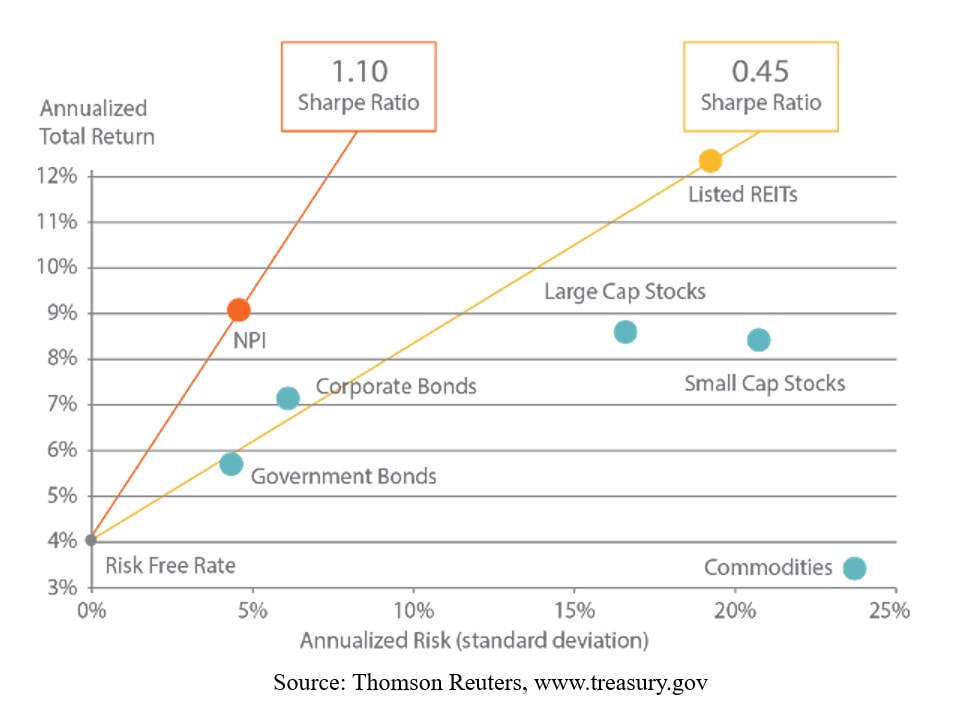
This "smoothness" is the inverse of risk or volatility. The Sharpe Ratio is a brilliant metric that formalizes this intuition by measuring the return you get per unit of risk taken.

To get a strong visual and conceptual grasp of this idea, the following video is an excellent starting point.

As the video explains, the Sharpe Ratio is calculated with the following formula:

Where:

• $R_p$ is the expected return of the portfolio.
• $R_f$ is the risk-free rate.
• ${\sigma }_p$ is the standard deviation of the portfolio's returns (its volatility).

The numerator, $R_p-R_f$, is the excess return: how much your portfolio earned above a "no-risk" investment. The Sharpe Ratio tells you how much excess return you generated for every unit of volatility you had to endure.

2. Calculating the Components for a Real Estate Portfolio

To calculate the Sharpe Ratio, we need to compute its three components: $R_p$, $R_f$, and ${\sigma }_p$.

A. Portfolio Expected Return ($R_p$)

This is the straightforward part. The expected return of your portfolio is the weighted average of the expected returns of its individual assets.

Where $w_i$ is the weight (percentage of the total portfolio value) of asset $i$, and $R_i$ is the expected return of asset $i$.

B. The Risk-Free Rate ($R_f$)

This is the theoretical return of an investment with zero risk. In practice, we use the yield on a long-term government bond from a stable country. For our purposes, the Spanish 10-year government bond yield is the appropriate benchmark. As of mid-2024, this rate is approximately 3.3%. We will use this value in our calculations.

C. Portfolio Volatility (${\sigma }_p$)

This is the most complex component and where our previous lesson on correlation becomes critical. The total risk of a portfolio is not simply the weighted average of the individual asset risks. The interaction between the assets—their correlation—plays a huge role.

A portfolio's variance (${\sigma }_p^2$, the square of its volatility) is calculated using matrix algebra, which elegantly combines individual asset variances and their covariances.

Where:

• $\mathbf{w}$ is the column vector of portfolio weights.
• ${\mathbf{w}}^T$ is the transpose of the weights vector.
• $\mathbf{\Sigma }$ (Sigma) is the covariance matrix of the assets' returns.

The covariance matrix $\mathbf{\Sigma }$ is the mathematical structure that holds all the risk information: the individual asset variances sit on its diagonal, and the covariances between each pair of assets fill the rest of the matrix. Since $\text{Cov}(i,j)={\rho }_{ij}{\sigma }_i{\sigma }_j$, this matrix is precisely how the correlations we calculated last lesson influence the total portfolio risk.

Combining assets with low or negative correlation reduces the off-diagonal values in the covariance matrix, leading to a lower overall portfolio variance (${\sigma }_p^2$) and thus lower volatility (${\sigma }_p$). This is the mathematical basis of diversification.

3. Python Implementation: Calculating the Sharpe Ratio

Let's now apply this by building a Python function. We will continue with the same three hypothetical assets from our previous lesson to maintain continuity.

First, let's assume we have our portfolio weights. For example, let's say we have a portfolio allocated as follows:

• 40% in Madrid Office
• 40% in Barcelona Apartment
• 20% in Valencia Logistics

Here is the complete Python code to calculate the portfolio return, volatility, and Sharpe Ratio.

import pandas as pd
import numpy as np

# 1. DATA SETUP
# Same hypothetical annual returns (%) from the previous lesson
data = {
    'Madrid_Office':    [3.0, 3.5, 4.0, 1.0, -1.0],
    'Barcelona_Apt':    [4.0, 4.5, 5.0, 2.5,  0.5],
    'Valencia_Logistic':[6.0, 7.0, 8.0, 9.0,  5.0]
}
returns_df = pd.DataFrame(data)

# Portfolio weights
weights = np.array([0.40, 0.40, 0.20]) # 40% Office, 40% Apt, 20% Logistic

# Risk-free rate (e.g., Spanish 10-year bond yield)
risk_free_rate = 0.033 # 3.3%

# 2. CALCULATE ANNUALIZED INPUTS
# We need returns as decimals, not percentages
returns_decimal = returns_df / 100

# Calculate annualized mean returns
# For annual data, mean() is already the annualized mean return.
# If we used daily/monthly data, we'd need to multiply by 252/12.
mean_returns = returns_decimal.mean()

# Calculate the annualized covariance matrix
cov_matrix = returns_decimal.cov()

# 3. CALCULATE PORTFOLIO METRICS
# Portfolio Expected Return (Annualized)
portfolio_return = np.sum(mean_returns * weights)

# Portfolio Volatility (Annualized)
# The formula is sqrt(w^T * Cov_Matrix * w)
portfolio_variance = np.dot(weights.T, np.dot(cov_matrix, weights))
portfolio_volatility = np.sqrt(portfolio_variance)

# 4. CALCULATE SHARPE RATIO
sharpe_ratio = (portfolio_return - risk_free_rate) / portfolio_volatility

# 5. DISPLAY RESULTS
print(f"Portfolio Allocation:")
for i, asset in enumerate(returns_df.columns):
    print(f"  - {asset}: {weights[i]:.0%}")

print("\n--- Annualized Performance ---")
print(f"Expected Return:    {portfolio_return:.2%}")
print(f"Volatility (Risk):  {portfolio_volatility:.2%}")
print(f"Risk-Free Rate:     {risk_free_rate:.2%}")
print("------------------------------")
print(f"Sharpe Ratio:       {sharpe_ratio:.2f}")

Output of the Code:

Portfolio Allocation:
  - Madrid_Office: 40%
  - Barcelona_Apt: 40%
  - Valencia_Logistic: 20%

--- Annualized Performance ---
Expected Return:    3.56%
Volatility (Risk):  2.34%
Risk-Free Rate:     3.30%
------------------------------
Sharpe Ratio:       0.11

Interpretation:
A Sharpe Ratio of 0.11 is very low. It indicates that for the risk taken, the portfolio is generating very little excess return over a safe government bond. This is mainly because the expected return (3.56%) is barely above the risk-free rate (3.30%). An investor might conclude that this particular portfolio is not worth the risk.

The code we wrote calculates the Sharpe Ratio for one specific set of weights. As a software engineer, you can see the next logical step: how do we find the optimal weights that give the maximum Sharpe Ratio? This process is called portfolio optimization.

For a detailed walkthrough of how to implement this using both Monte Carlo simulation (trying thousands of random weights) and direct mathematical optimization with SciPy, the following article is an excellent practical guide.

Conclusion

You have now learned to calculate one of the most important metrics in all of finance. The Sharpe Ratio allows you to distill a portfolio's complex behavior—its returns, its individual asset risks, and the intricate correlations between them—into a single, comparable number. It is the ultimate measure of investment efficiency.

Key Takeaways:

• Risk-adjusted return is a measure of how much return an investment generates for the amount of risk taken.
• The Sharpe Ratio is the primary metric for this, calculated as $(R_p-R_f)/{\sigma }_p$.
• A higher Sharpe Ratio is always better, indicating a more efficient portfolio.
• Portfolio volatility (${\sigma }_p$) is the most complex component, as it depends on both individual asset volatilities and the correlation between them.
• We can implement the calculation in Python using NumPy for the matrix mathematics required to compute portfolio volatility.

Preview of the Next Lesson:
With the ability to calculate HHI, correlation, and now the Portfolio Sharpe Ratio, we have completed our analytical toolkit. In our next lesson, we will move from analysis to synthesis. The learning outcome will be to define a framework for building a diversified real estate portfolio in Spain. We will discuss how to set investment goals and constraints and use these powerful metrics to strategically select and weight assets to construct a portfolio that is optimized for your specific objectives.