Single-Asset Financial Model with Tax & Risk in Python

Hello! Welcome to our second-to-last lesson.

In our previous session, we established a high-level strategic framework for building a diversified real estate portfolio in Spain. We covered the five essential steps, from defining your goals to monitoring and rebalancing. You learned that the third step, Tactical Asset Selection, involves a deep, "bottom-up" analysis of individual properties.

Today, we're going to build the engine for that analysis. Our goal is to develop a comprehensive Python model that integrates financial projections, multi-faceted tax calculations, and key risk/return metrics for a single asset. This lesson is the culmination of nearly everything we've studied, combining income, expenses, financing, valuation, risk, and—most importantly—the specifics of Spanish taxation into a single, powerful tool. For someone with your software engineering background, this is where all the concepts translate into a tangible, reusable structure.

The Anatomy of a Single-Asset Model

Think of this model as a blueprint for evaluating any potential real estate deal. A well-structured model should be able to take a set of inputs about a property and produce a clear set of outputs that inform your investment decision. Given your background, we'll design this using an object-oriented approach in Python, creating a class to represent a property investment.

Our model will have four main components:

1. Inputs & Assumptions: The raw data about the deal.
2. Pro-Forma Projections: A multi-year forecast of financial performance.
3. Spanish Tax Calculations: The specific tax liabilities on income and capital gains.
4. Metric Outputs: The final quantitative results (IRR, NPV, etc.) that summarize the investment's potential.

Let's break down each component.

1. Inputs & Assumptions: The Data Layer

Every analysis starts with data. Our model needs a comprehensive set of inputs to function. We can structure these as parameters we pass when creating an instance of our RealEstateAsset class.

Purchase & Sale:

• purchase_price: The agreed-upon price of the property.
• closing_costs_pct: Percentage of the purchase price for fees (notary, registry) and taxes like ITP or IVA.
• holding_period_years: How long you plan to own the property.
• exit_cap_rate: The expected cap rate at the time of sale, used to project the sale price.

Financing (from Module 2):

• loan_to_value_ratio: The percentage of the purchase price financed by a mortgage.
• interest_rate: The annual interest rate on the loan.
• loan_term_years: The amortization period of the loan.

Operations (from Modules 1 & 5):

• gross_monthly_rent: Initial rent collected.
• annual_rent_growth: The assumed yearly percentage increase in rent.
• vacancy_rate: Percentage of gross rent lost to vacancy.
• operating_expenses_pct: Operating expenses (maintenance, insurance, IBI, etc.) as a percentage of gross operating income.
• annual_opex_growth: Assumed yearly growth in operating expenses.
• capex_reserve_pct: Percentage of gross rent set aside for capital expenditures.

Spanish Tax Parameters (from Modules 9 & 10):

• property_value_for_depreciation: The value base for tax depreciation (valor de adquisición or valor catastral).
• irpf_rental_income_rate: Your marginal IRPF tax rate for ordinary income.
• irpf_capital_gains_rate: Your marginal IRPF tax rate for capital gains.
• irpf_rental_reduction_pct: The specific reduction on net rental income (e.g., 50% for general cases, up to 90% in tensioned zones).

2. Pro-Forma Projections: The Financial Forecast

The core of our model is the pro-forma, a multi-year cash flow statement. We can represent this perfectly using a pandas DataFrame, where each row is a line item and each column is a year in our holding period.

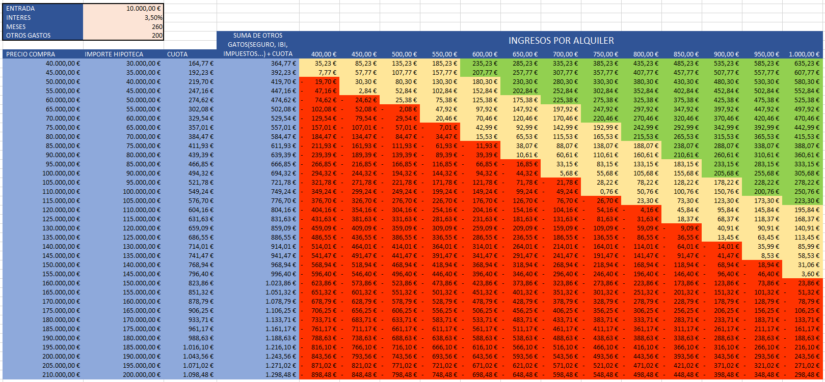
The logic flows sequentially, just as we learned in the early modules:

1. Potential Gross Income (PGI): gross_monthly_rent * 12, grown annually by annual_rent_growth.
2. Vacancy Loss: PGI * vacancy_rate.
3. Effective Gross Income (EGI): PGI - Vacancy Loss.
4. Operating Expenses (OpEx): EGI * operating_expenses_pct, grown annually.
5. Net Operating Income (NOI): EGI - OpEx.
6. Debt Service: The total annual mortgage payments (principal + interest). We can pre-calculate this using an amortization schedule function.
7. Pre-Tax Cash Flow (CFBT): NOI - Debt Service. Note: We typically add the CapEx reserve back here if it was included in OpEx, as it's not a true cash expense in that year. A more precise approach is to subtract it from NOI to get NOI - CapEx Reserve, and then subtract debt service. For our model, we'll keep it simple: CFBT = NOI - Debt Service.

3. Spanish Tax Calculations: The Critical Layer

This is where the model becomes truly valuable and tailored to your context. We need to implement the specific rules from Modules 9 and 10.

Annual Rental Income Tax (IRPF)

For each year of the projection, we calculate the tax on rental income. To do this properly, you must first understand which expenses are deductible.

Based on that reading, our model will perform these steps for each year:

1. Calculate Net Rental Yield (Rendimiento Neto): This is Gross Rental Income - All Deductible Expenses. The main deductible expenses are:

   • Operating Expenses (IBI, community fees, insurance, etc.).
   • Mortgage Interest (not principal).
   • Amortización (Depreciation): property_value_for_depreciation * 0.03.

2. Apply Reduction: Multiply the Net Rental Yield by the applicable reduction (e.g., 50%).

   • Taxable Base = Net Rental Yield * (1 - irpf_rental_reduction_pct)

3. Calculate IRPF on Rental Income: Tax on Income = Taxable Base * irpf_rental_income_rate.

4. Calculate After-Tax Cash Flow (CFAT): Pre-Tax Cash Flow (CFBT) - Tax on Income.

Taxes on Sale

At the end of the holding period, we calculate the taxes due on the property's disposition:

1. Projected Sale Price: (Year N+1 NOI) / exit_cap_rate.
2. Calculate Capital Gain: Sale Price - Adjusted Acquisition Cost.
3. Calculate IRPF on Capital Gain: Capital Gain * irpf_capital_gains_rate.
4. Calculate After-Tax Reversion: Sale Price - Sale Costs - Remaining Loan Balance - IRPF on Capital Gain. (We'll omit Plusvalía Municipal for simplicity in this model, but a full version would include it).

4. Metric Outputs & Python Implementation

With all cash flows calculated, we can now compute the final metrics. The most important step is to construct the full cash flow stream for the investment:

• Year 0: The initial investment (a negative number). This is -(Purchase Price * (1 - LTV) + Purchase Price * Closing Costs %).
• Year 1 to N-1: The annual After-Tax Cash Flow (CFAT).
• Year N: The final year's CFAT + the After-Tax Reversion from the sale.

With this list of cash flows, we can use the numpy_financial library to get our final answers.

A common pitfall is to try to calculate IRR on an incorrect series of values. This Stack Overflow thread is a perfect illustration of why constructing the complete net cash flow stream is essential.

Python Code Structure

Here is a skeleton of what our RealEstateAsset class could look like. It encapsulates the logic we've discussed.

import pandas as pd
import numpy_financial as npf

class RealEstateAsset:
    def __init__(self, **inputs):
        self.inputs = inputs
        self.pro_forma = None
        self.metrics = {}

    def generate_pro_forma(self):
        # Logic to build the pandas DataFrame for the pro-forma.
        # It will have rows for PGI, EGI, OpEx, NOI, Debt Service, etc.
        # And columns for each year of the holding period.
        # ...
        print("Pro-forma generated.")
        # self.pro_forma = ...
    
    def calculate_taxes(self):
        # Requires self.pro_forma to be generated first.
        # Loop through each year in the pro-forma DataFrame.
        # Calculate taxable rental income (Rendimiento Neto).
        # Apply IRPF reduction.
        # Calculate annual tax and After-Tax Cash Flow.
        # Calculate taxes on sale at the end of the holding period.
        # ...
        print("Taxes calculated.")

    def calculate_metrics(self):
        # Requires taxes to be calculated.
        # 1. Construct the final after-tax cash flow list/array.
        #    - Initial Investment (negative)
        #    - Annual CFATs
        #    - Final CFAT + After-Tax Reversion
        
        # 2. Use numpy-financial to calculate metrics.
        # cash_flows = [...]
        # self.metrics['irr'] = npf.irr(cash_flows)
        # self.metrics['npv'] = npf.npv(self.inputs['discount_rate'], cash_flows)
        # ...
        print("Metrics calculated.")

    def run_analysis(self):
        self.generate_pro_forma()
        self.calculate_taxes()
        self.calculate_metrics()
        return self.pro_forma, self.metrics

# Example Usage:
# property_inputs = { 'purchase_price': 200000, ... }
# my_property = RealEstateAsset(**property_inputs)
# pro_forma_df, final_metrics = my_property.run_analysis()
# print(final_metrics)

Conclusion

Today we've designed the blueprint for a comprehensive, single-asset financial model tailored specifically for the Spanish real estate market. This is the ultimate "bottom-up" analysis tool that forms the core of any serious investment process.

Key Takeaways:

• A robust model is structured into four parts: Inputs, Projections (Pro-Forma), Tax Calculations, and Metrics.
• Using a Python class is an excellent way to encapsulate the logic and make the model reusable.
• The pro-forma is a multi-year forecast that builds from Gross Income down to Pre-Tax Cash Flow.
• The Spanish tax layer is what makes the model powerful, accurately calculating Rendimiento Neto by including deductions like mortgage interest and depreciation, and applying the correct IRPF reductions.
• The final step is to construct the complete after-tax cash flow stream (including the initial investment) to correctly calculate metrics like IRR and NPV using libraries like numpy-financial.

Preview of the Next Lesson:
This single-asset model gives us the expected after-tax return (IRR) and risk for one investment. In our final lesson, we will learn how to use the outputs from several of these models to perform a portfolio optimization. We will combine multiple assets, consider their correlations, and find the optimal allocation to build a diversified portfolio that maximizes risk-adjusted returns, bringing our entire course to a powerful conclusion.