Optimizing Spanish Property Portfolios: After-Tax Risk & Return

Hello! Welcome to the final lesson of our course on real estate investment analysis.

In our previous lesson, we built a powerful, comprehensive Python model to analyze a single real estate asset. That model integrated financial projections, complex Spanish tax calculations, and risk metrics to produce key outputs like the after-tax Internal Rate of Return (IRR) and Net Present Value (NPV). This gave us a robust "bottom-up" method for evaluating the merits of any individual deal.

Now, we will take the final and most strategic step. An investor's goal is rarely to find just one good property, but to build a portfolio of properties that work together to maximize returns while managing risk. This lesson directly addresses that challenge. Our learning outcome is to write Python code to implement a basic portfolio allocation optimization for multiple Spanish properties based on after-tax risk and return metrics.

We will use the principles of Modern Portfolio Theory (MPT), a Nobel Prize-winning framework, and adapt them to the unique characteristics of real estate. For you as a software engineer, this lesson will feel like a classic optimization problem: finding an optimal solution within a set of constraints. We'll translate financial theory into practical Python code to determine the ideal investment allocation across several properties.

Let's begin this culminating lesson.

1. From Single Assets to a Portfolio: Modern Portfolio Theory (MPT)

Modern Portfolio Theory, developed by Harry Markowitz, provides a mathematical framework for building diversified investment portfolios. Its central idea is that the risk of a portfolio is not just the average risk of its assets, but a function of how their returns move in relation to one another.

Here are the core components:

• Expected Return: The portfolio's expected return is simply the weighted average of the expected returns of the individual assets.
• Risk (Volatility): The portfolio's risk, measured by standard deviation, is more complex. It depends on the individual assets' risk and the correlation between them.
• Correlation: A measure of how two assets' returns move together. It ranges from +1 (perfectly correlated) to -1 (perfectly uncorrelated). The power of diversification comes from combining assets with low or negative correlation.

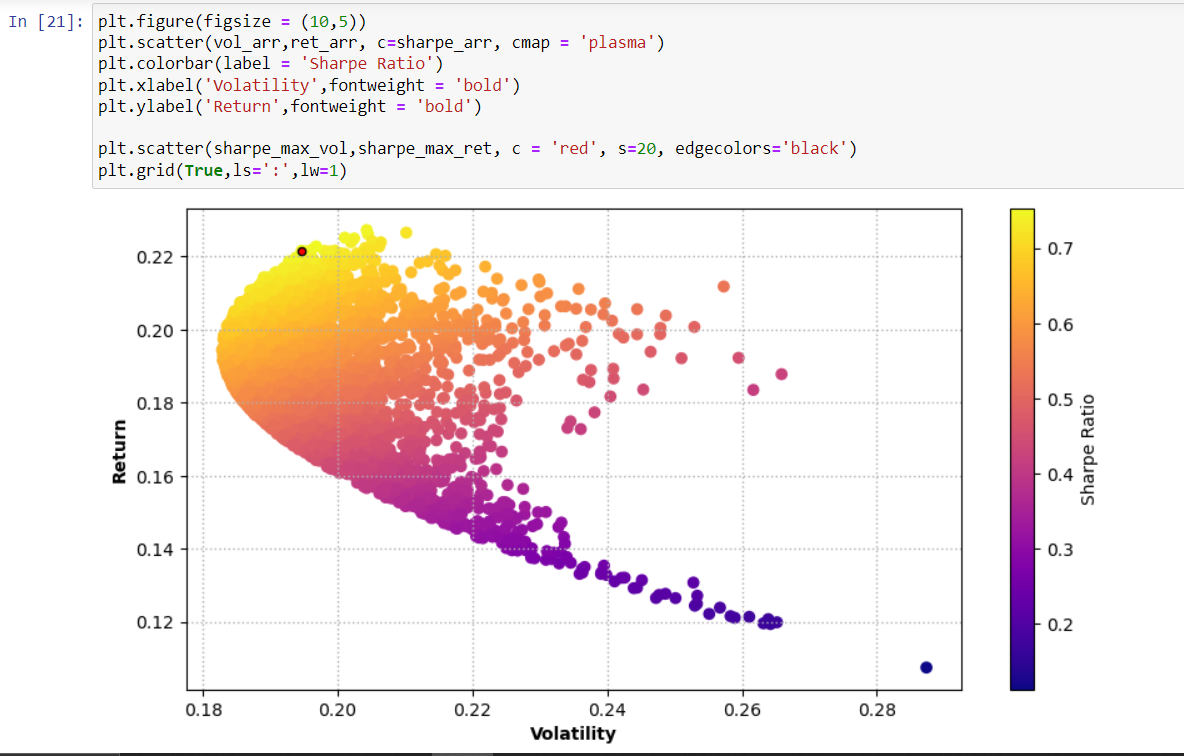
The goal of MPT is to find the Efficient Frontier: a curve representing the set of optimal portfolios that offer the highest expected return for a given level of risk.

2. Adapting MPT for Real Estate

While MPT was developed for liquid assets like stocks, we can adapt its principles for real estate. The main challenge is sourcing the inputs. For stocks, we can use years of historical price data. For real estate, data is scarcer, so we must rely on the models and estimates we've developed throughout this course.

Here's how we'll source our inputs for the MPT model:

1. Expected Return ($\mu$): For each property, we'll use the after-tax IRR calculated from the single-asset model we designed in the last lesson. This is our best estimate of the property's long-term annualized return.
2. Risk ($\sigma$): This is the expected volatility (standard deviation) of the return. We can't easily get this from historical data. A practical approach is to run a sensitivity or scenario analysis on our single-asset model. By modeling 'best-case', 'base-case', and 'worst-case' scenarios for variables like rent growth and exit cap rate, we can generate a distribution of possible IRRs and calculate the standard deviation.
3. Correlation ($\rho$): This is the most subjective input. We must estimate the correlation between properties based on qualitative factors. For instance:
   • Two apartments in the same building in Madrid: High correlation (e.g., 0.8). Their values will likely move in lockstep.
   • A retail unit in Barcelona and a residential flat in Valencia: Moderate correlation (e.g., 0.4). They are in different cities and sectors.
   • An industrial warehouse in a logistics hub and a rural holiday home: Low correlation (e.g., 0.1). Their performance is driven by very different economic factors.

With these estimated inputs—expected returns, standard deviations, and correlations—we can build the covariance matrix, a key ingredient for the portfolio risk calculation. The covariance between two assets $i$ and $j$ is given by:

$\text{Cov}(i,j)={\rho }_{ij}\cdot {\sigma }_i\cdot {\sigma }_j$

Where ${\rho }_{ij}$ is the correlation between $i$ and $j$, and ${\sigma }_i$ and ${\sigma }_j$ are their respective standard deviations.

3. Implementing Portfolio Optimization in Python

We will now implement an MPT model in Python. The process involves two main stages: simulating many random portfolios to visualize the risk-return universe, and then using an optimizer to find the single best portfolio.

The following resource provides an excellent, detailed guide on how to do this using standard Python libraries. We will follow its structure, adapting the context from stocks to our real estate assets.

Step-by-Step Python Implementation

Let's walk through the code. We'll assume we have analyzed three potential properties using our single-asset model and have the following after-tax risk/return estimates.

1. Define Asset Inputs

First, we set up our inputs: expected returns (IRRs), risks (standard deviations), and our estimated correlation matrix.

import numpy as np
import pandas as pd
import scipy.optimize as sco

# --- INPUTS ---
# These would come from our single-asset models
# Property A: Residential Flat, Madrid Center
# Property B: Commercial Local, Valencia
# Property C: Industrial Warehouse, Zaragoza
assets = ['Property_A', 'Property_B', 'Property_C']
expected_returns = np.array([0.08, 0.065, 0.09])  # After-tax IRR
risks = np.array([0.12, 0.10, 0.15]) # Standard Deviation of IRR

# Estimated Correlation Matrix
correlation_matrix = np.array([
    [1.0, 0.4, 0.2],  # A->A, A->B, A->C
    [0.4, 1.0, 0.5],  # B->A, B->B, B->C
    [0.2, 0.5, 1.0]   # C->A, C->B, C->C
])

# Calculate the Covariance Matrix
covariance_matrix = np.outer(risks, risks) * correlation_matrix

2. Portfolio Return and Risk Functions

Next, we define functions to calculate the expected return and standard deviation for a portfolio with a given set of weights.

# Function to calculate annualized portfolio return
def portfolio_return(weights, returns):
    return np.sum(returns * weights)

# Function to calculate annualized portfolio volatility (risk)
def portfolio_risk(weights, cov_matrix):
    return np.sqrt(np.dot(weights.T, np.dot(cov_matrix, weights)))

3. Finding the Optimal Portfolio (Maximum Sharpe Ratio)

Our primary goal is to find the portfolio with the best risk-adjusted return. We use the Sharpe Ratio for this, which is (Portfolio Return - Risk-Free Rate) / Portfolio Risk. For simplicity, we'll assume a risk-free rate of 0.

We'll use scipy.optimize.minimize to find the weights that maximize this ratio. Since minimize finds a minimum, we'll tell it to minimize the negative Sharpe Ratio.

def negative_sharpe_ratio(weights, returns, cov_matrix, risk_free_rate=0.0):
    p_return = portfolio_return(weights, returns)
    p_risk = portfolio_risk(weights, cov_matrix)
    return -(p_return - risk_free_rate) / p_risk

# --- Optimization ---
num_assets = len(assets)

# Constraints: weights must sum to 1
constraints = ({'type': 'eq', 'fun': lambda weights: np.sum(weights) - 1})

# Bounds: weights must be between 0 and 1
bounds = tuple((0, 1) for asset in range(num_assets))

# Initial guess: equal weights
initial_weights = np.array(num_assets * [1. / num_assets,])

# Run the optimization
optimal_portfolio_result = sco.minimize(
    negative_sharpe_ratio, 
    initial_weights, 
    args=(expected_returns, covariance_matrix), 
    method='SLSQP', 
    bounds=bounds, 
    constraints=constraints
)

# Get the optimal weights
optimal_weights = optimal_portfolio_result.x

4. Displaying the Results

Finally, let's display the outcome of our optimization.

print("Optimal Portfolio Allocation:")
for i, weight in enumerate(optimal_weights):
    print(f"  - {assets[i]}: {weight:.2%}")

print("-" * 30)

opt_return = portfolio_return(optimal_weights, expected_returns)
opt_risk = portfolio_risk(optimal_weights, covariance_matrix)
opt_sharpe = -optimal_portfolio_result.fun # a.k.a. (opt_return / opt_risk)

print(f"Expected Annual Return: {opt_return:.2%}")
print(f"Expected Annual Volatility (Risk): {opt_risk:.2%}")
print(f"Sharpe Ratio: {opt_sharpe:.2f}")

# Example Output:
# Optimal Portfolio Allocation:
#   - Property_A: 44.59%
#   - Property_B: 43.10%
#   - Property_C: 12.31%
# ------------------------------
# Expected Annual Return: 7.64%
# Expected Annual Volatility (Risk): 9.39%
# Sharpe Ratio: 0.81

This output gives us a clear, actionable investment strategy based on our analysis: allocate our capital across the three properties according to these optimal weights to achieve the best possible risk-adjusted return.

4. An Alternative View: Linear Programming

The MPT approach we just used is a form of Quadratic Programming because the risk function involves squared terms. An alternative, simpler approach is to frame the problem as a Linear Program (LP). This is something your software engineering background might find very intuitive, as it's a common type of problem in computer science.

In an LP formulation, we can maximize the portfolio return subject to a set of linear constraints, including a hard cap on total portfolio risk.

This LP approach is less common for pure risk-return optimization than MPT but is extremely flexible for adding business rules, such as "do not invest more than 50% in any single property" or "ensure at least 20% of the portfolio is in residential assets."

Conclusion and Course Wrap-Up

Today, we've reached the pinnacle of our quantitative journey. We took the detailed outputs from our single-asset models and used them as inputs for a sophisticated portfolio optimization framework. This allows us to move from analyzing deals in isolation to building a strategic, diversified real estate portfolio.

Key Takeaways:

• Modern Portfolio Theory (MPT) provides a mathematical framework to maximize return for a given level of risk by combining assets with different risk-return profiles and correlations.
• For real estate, the key inputs for MPT (expected return, risk, and correlation) must be carefully estimated using our single-asset financial models and qualitative judgment.
• Using Python libraries like numpy and scipy.optimize, we can implement an optimizer to find the optimal portfolio weights that maximize the risk-adjusted return (Sharpe Ratio).
• The final output is a concrete, data-driven allocation strategy, guiding how to distribute capital across multiple investment opportunities.

This lesson concludes our course. We have journeyed from the foundational definitions of income and expenses to the complexities of Spanish taxation and, finally, to portfolio-level optimization. You have built a complete, end-to-end quantitative skillset for analyzing real estate investments in Spain, grounded in practical coding and real-world application.

Your path as an investor is one of continuous learning. The models and frameworks we have developed are powerful tools, but they should always be combined with on-the-ground market knowledge, thorough due diligence, and sound judgment. Congratulations on completing this intensive course