Vector Database Indexing and Retrieval

Introduction

In our last lesson, we established how to measure the semantic relatedness between two text embeddings using cosine similarity. The key takeaway was that while this works perfectly for a pair of vectors, it becomes computationally infeasible when you need to compare a query vector against millions or even billions of vectors in a database. A one-by-one comparison, known as a brute-force search, is simply too slow.

This lesson directly addresses that challenge. Our goal is to describe how vector databases index and retrieve embeddings efficiently. We'll move beyond simple pairwise comparisons and explore the clever data structures and algorithms that make large-scale semantic search possible.

We will cover:

• The problem with brute-force search and why it doesn't scale.
• The core concept of Approximate Nearest Neighbor (ANN) search, the fundamental trade-off that underpins modern vector search.
• The main families of indexing algorithms, focusing on the two most important ones: Inverted File (IVF) and Hierarchical Navigable Small World (HNSW).
• The role of Product Quantization (PQ) in compressing vectors to manage memory usage.

By the end of this lesson, you will understand the architectural principles that allow vector databases to find the "good enough" closest matches from a massive collection of vectors in milliseconds.

The Problem: Brute-Force Search and the "Flat" Index

The simplest way to find the nearest neighbors to a query vector is to compute its similarity score (e.g., cosine similarity) with every single vector in your database. This approach is called a brute-force search, and the corresponding index is often called a "flat" index because it involves no special organization of the vectors.

As the video explains, if you have $N$ vectors and each vector has $d$ dimensions, a single search requires $N$ distance calculations. The complexity is $O(N\times d)$. While this might be acceptable for a few thousand vectors, it quickly becomes a bottleneck for the millions or billions of embeddings common in real-world applications.

The Solution: Approximate Nearest Neighbor (ANN) Search

To overcome the limitations of brute-force search, vector databases use Approximate Nearest Neighbor (ANN) algorithms. The core idea is a classic engineering trade-off: sacrifice a small amount of accuracy to gain a massive improvement in search speed.

Instead of guaranteeing the exact top-K nearest neighbors, ANN algorithms aim to find vectors that are very close to the true nearest neighbors, with high probability. For most applications, like semantic search or RAG, the difference between the absolute best match and the 99th-percentile best match is negligible.

This trade-off is necessary because of a phenomenon known as the "curse of dimensionality." In high-dimensional spaces (like the 768 or 1536 dimensions of typical embeddings), traditional indexing structures like k-d trees become inefficient, and the concept of distance itself becomes less intuitive. ANN algorithms are specifically designed to navigate these high-dimensional spaces efficiently.

Core Indexing Strategies

Vector databases employ several families of ANN algorithms to structure the data for fast retrieval. Let's explore the most important ones.

1. Cluster-Based Indexing: Inverted File (IVF)

The Inverted File (IVF) index works by partitioning your vector space into a predefined number of clusters.

1. Build Phase: A clustering algorithm (like k-means) is run on a sample of the data to find a set of representative points called centroids. The entire vector space is now divided into partitions, or "cells," one for each centroid. Each vector in the database is then assigned to its nearest centroid.
2. Search Phase: When a query vector arrives, the system first finds the few closest centroids to the query (a parameter called nprobe). Instead of searching the entire dataset, it only searches the vectors within the cells corresponding to those selected centroids.

This is analogous to searching for a book in a library: instead of checking every single book, you first go to the correct section (e.g., "Computer Science"), dramatically narrowing your search space.

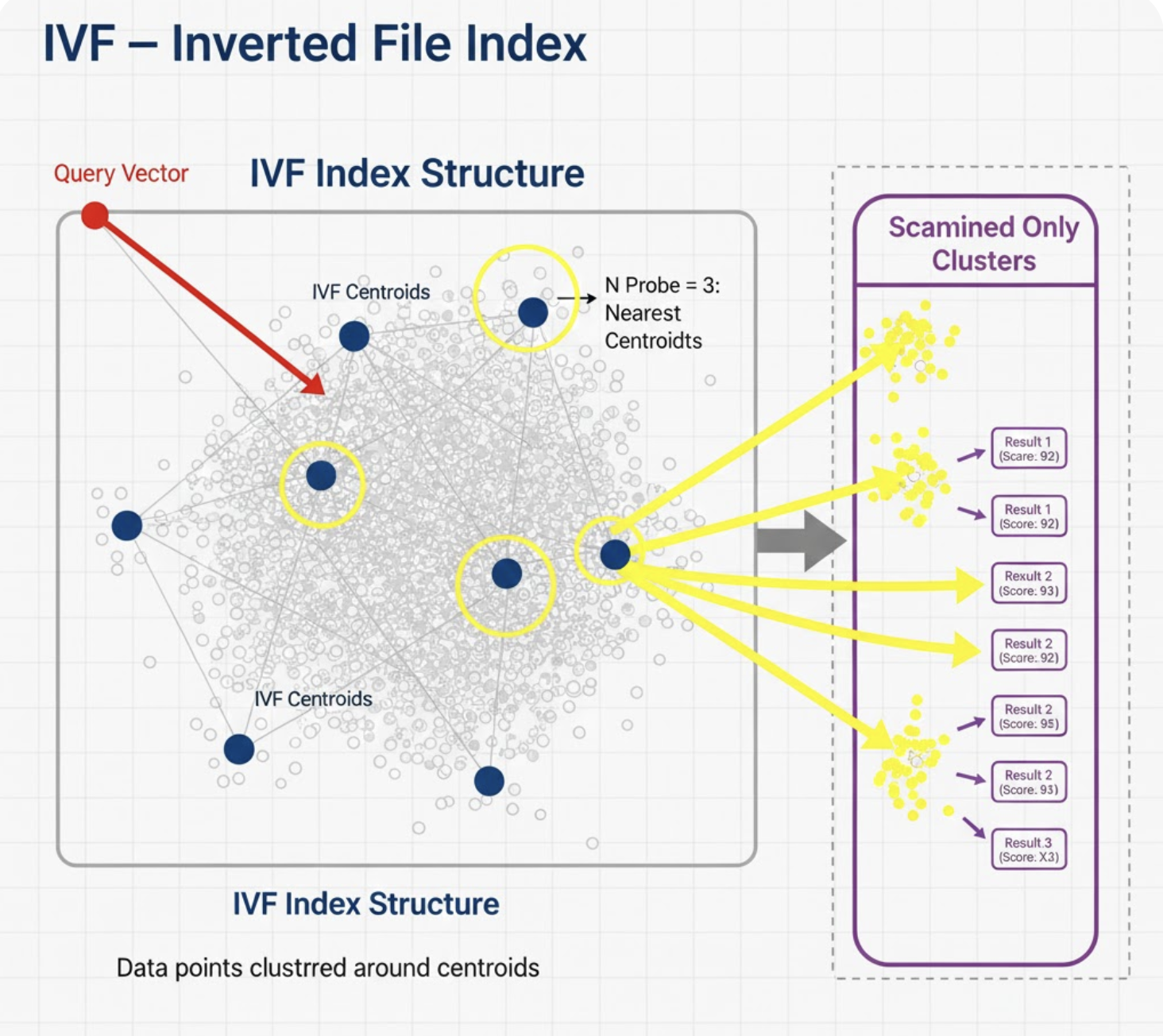
The main trade-off with IVF is between speed and recall, controlled by the nprobe parameter. A larger nprobe means searching more clusters, which is slower but more likely to find the true nearest neighbors.

2. Graph-Based Indexing: HNSW (Hierarchical Navigable Small World)

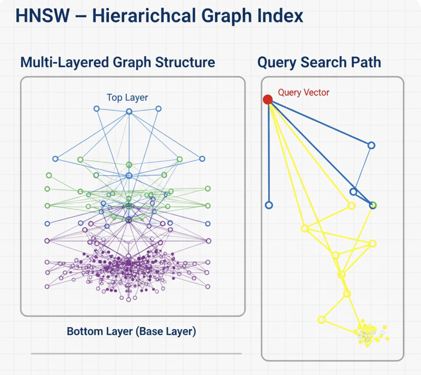
HNSW is currently one of the most popular and effective ANN algorithms, known for its excellent speed and accuracy. It builds a graph where vectors are nodes and edges connect vectors that are close to each other.

The "Hierarchical" part is the key innovation:

1. Build Phase: HNSW creates a multi-layered graph. The top layers are sparse, containing only a few nodes with long-range connections that act like a "highway system" for the search. Each subsequent layer becomes progressively denser, with more nodes and shorter-range connections, like local roads. The bottom layer contains all the vectors.
2. Search Phase: A search starts at an entry point in the sparsest top layer. The algorithm greedily traverses the graph, always moving to the neighbor closest to the query vector. Once it can't find a closer neighbor in the current layer, it drops down to the next, denser layer and continues the search. This process repeats until it reaches the bottom layer, where it performs a fine-grained local search.

To understand this process in more detail, let's watch a video that explains both IVF and HNSW.

HNSW generally provides the best balance of performance and accuracy, which is why it's the default index in many modern vector databases like Pinecone, Weaviate, and Milvus.

3. Vector Compression: Product Quantization (PQ)

While IVF and HNSW solve the problem of search speed, Product Quantization (PQ) addresses the problem of memory. A single 1536-dimensional embedding using 32-bit floats takes up 6KB of memory. Storing a billion of these would require 6TB of RAM, which is infeasible for many systems.

PQ is a compression technique that dramatically reduces memory usage:

1. The high-dimensional vector is split into several smaller sub-vectors.
2. For each set of sub-vectors, a separate k-means clustering is performed to create a small "codebook" of centroids.
3. Each original sub-vector is then replaced by the ID of its closest centroid in the codebook.

For example, a 128-dimensional vector can be split into 8 sub-vectors of 16 dimensions each. If each codebook has 256 centroids, each 16-dimensional sub-vector can be represented by a single byte (since $2^8=256$). The entire 128-dimensional vector is now compressed from 512 bytes (128 * 4 bytes) to just 8 bytes.

PQ is rarely used alone. It is most powerful when combined with an index like IVF, creating an IVF-PQ index. In this setup, IVF provides the coarse search structure (the inverted lists), and within each list, the vectors are stored in their compressed PQ form. This allows for both fast search and a very low memory footprint.

Performance Comparison and Real-World Systems

As a software engineer, you'll naturally think about the trade-offs. Each indexing strategy has different characteristics regarding build time, query speed, memory usage, and accuracy (recall).

The following resource provides an excellent summary table comparing the different index types.

In practice, modern vector databases often use hybrid indexes that combine the strengths of multiple approaches (e.g., using HNSW on compressed PQ vectors) to optimize for specific workloads. They also provide all the other features you'd expect from a database system:

• Scalability through sharding and replication.
• Metadata storage and filtering (e.g., "find documents similar to X, but only from category='tutorial'").
• Data durability and standard CRUD (Create, Read, Update, Delete) operations.

These features transform a standalone ANN library into a robust, scalable backend for AI applications.

Conclusion

In this lesson, we've demystified how vector databases perform efficient similarity search at scale.

Key Takeaways:

• Brute-force ("flat") search is 100% accurate but too slow for large datasets, with a complexity of $O(N\times d)$.
• The solution is Approximate Nearest Neighbor (ANN) search, which trades a small amount of accuracy for huge gains in speed.
• IVF (Inverted File) is a cluster-based index that partitions the data and only searches a few relevant partitions, making it fast and memory-efficient.
• HNSW (Hierarchical Navigable Small World) is a graph-based index that builds a multi-layered navigation structure, offering state-of-the-art performance for many use cases.
• Product Quantization (PQ) is a vector compression technique that significantly reduces memory usage, often combined with IVF to create IVF-PQ indexes for billion-scale datasets.
• A vector database combines these powerful indexing algorithms with traditional database features like scalability, metadata filtering, and data management.

You now have a solid conceptual understanding of the "magic" behind fast semantic search. In the next lesson, we will put this theory into practice. You'll set up a vector store (ChromaDB) and perform a similarity search on a corpus of documents, completing the full cycle from text to efficient retrieval.