Measuring Text Relatedness with Cosine Similarity

Introduction

In our last lesson, you learned how to generate text embeddings—the numerical vector representations of text—using both cloud APIs and local models. We've successfully converted raw text into a format that machines can understand.

This lesson addresses the next logical question: Now that we have these vectors, how do we use them to measure how similar two pieces of text are? The learning outcome for this session is to compute cosine similarity between embeddings to measure text relatedness.

We will cover:

1. The core concept of cosine similarity and what the resulting scores mean.
2. The underlying mathematics at a high, intuitive level.
3. How to compute it in Python, connecting it to your practical software engineering background.
4. Why this metric is the standard for comparing text embeddings.

By the end of this lesson, you'll be able to take any two text embeddings and calculate a meaningful score that quantifies their semantic relationship, a fundamental building block for semantic search and Retrieval-Augmented Generation (RAG).

What is Cosine Similarity? The Angle of Meaning

Imagine two vectors in space. Cosine similarity doesn't care about their length (or magnitude), only the angle between them.

• If two vectors point in the same direction, the angle between them is 0°, and their cosine similarity is 1. They are considered very similar.
• If they are perpendicular (orthogonal), the angle is 90°, and their cosine similarity is 0. They are considered unrelated.
• If they point in opposite directions, the angle is 180°, and their cosine similarity is -1. They are dissimilar.

For text embeddings, we typically deal with values between 0 and 1, as embeddings are rarely constructed to be perfectly opposite.

For a clear and intuitive explanation of this idea, please watch the following video from StatQuest. It uses a simple 2D example to build up the concept.

The key insight is that cosine similarity is immune to differences in magnitude. In the video's example, the phrases "hello" and "hello hello hello" have the same cosine similarity to "hello world" because they point in the same direction, even though their vector lengths are different. For text, this is powerful because it means a short document and a long document can be considered similar if they are about the same topic.

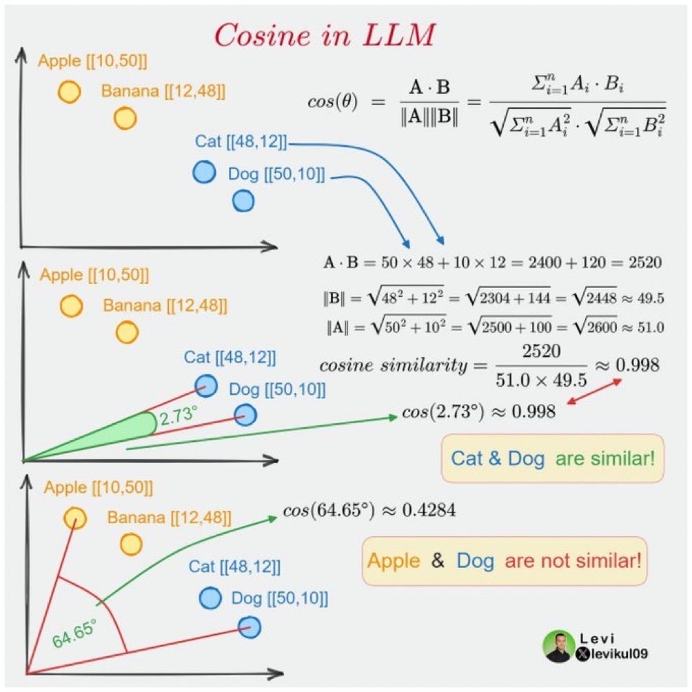
The image below provides another excellent visual summary, showing vectors for words. Notice the small angle (high similarity) between "Cat" and "Dog" and the large angle (low similarity) between "Apple" and "Dog".

The Mathematics Behind the Angle

While we don't need a deep mathematical dive, it's useful to understand the formula to see what's happening under the hood. The formula for the cosine similarity between two vectors, $\mathbf{A}$ and $\mathbf{B}$, is:

$$\text{Cosine Similarity}=\frac{\mathbf{A}\cdot \mathbf{B}}{\Vert \mathbf{A}\Vert \Vert \mathbf{B}\Vert }=\frac{{\sum }_{i=1}^n{A}_i{B}_i}{\sqrt{{\sum }_{i=1}^n{A}_i^2}\sqrt{{\sum }_{i=1}^n{B}_i^2}}$$

Let's break this down:

1. Numerator ($\mathbf{A}\cdot \mathbf{B}$): This is the dot product of the two vectors. You calculate it by multiplying corresponding components of the vectors and summing the results. The dot product is a single number that captures how much the two vectors "point in the same direction."

2. Denominator ($\Vert \mathbf{A}\Vert \Vert \mathbf{B}\Vert$): This is the product of the magnitudes (or lengths) of the two vectors. The magnitude is calculated using the Euclidean norm, which is essentially the Pythagorean theorem in higher dimensions. This part of the formula acts as a normalization factor, scaling the result to be between -1 and 1, thereby removing the influence of the vectors' lengths.

A Critical Shortcut for Modern LLMs

Here is a crucial insight for practical application. Most modern embedding models, including those from OpenAI, Cohere, and sentence-transformers, produce normalized vectors. This means the vectors are pre-scaled so that their magnitude is always 1.

When $\Vert \mathbf{A}\Vert =1$ and $\Vert \mathbf{B}\Vert =1$, the denominator in our formula becomes $1\times 1=1$. The formula simplifies to:

$$\text{Cosine Similarity}=\mathbf{A}\cdot \mathbf{B}$$

This means that for normalized embeddings, cosine similarity is simply the dot product. This is a significant optimization, as calculating the dot product is computationally cheaper than the full cosine similarity formula. Many vector databases and libraries leverage this fact.

The following video emphasizes this exact point.

Calculating Cosine Similarity in Python

Now let's get practical. As a software engineer, you'll want to know how to implement this. We'll use two sample embeddings that you could have generated in the previous lesson.

First, you'll need numpy and scikit-learn.

pip install numpy scikit-learn

Let's assume we have embeddings for two sentences:

• "The engineer writes clean code."
• "Software developers value good architecture."

These are semantically related, so we expect a high similarity score.

import numpy as np
from sklearn.metrics.pairwise import cosine_similarity




# Dummy 3D embeddings for demonstration. Real embeddings have many more dimensions.
# In a real scenario, you'd generate these with a model.
embedding_A = np.array([0.8, 0.4, 0.2]) # Represents "The engineer writes clean code."
embedding_B = np.array([0.7, 0.5, 0.1]) # Represents "Software developers value good architecture."




# Make sure they are normalized (magnitude of 1) to mimic real-world models.
embedding_A = embedding_A / np.linalg.norm(embedding_A)
embedding_B = embedding_B / np.linalg.norm(embedding_B)

print(f"Embedding A (normalized): {embedding_A}")
print(f"Embedding B (normalized): {embedding_B}")

Method 1: Manual Calculation with NumPy

This approach mirrors the formula and is great for understanding the mechanics.

# 1. Calculate the dot product
dot_product = np.dot(embedding_A, embedding_B)




# 2. Calculate the magnitudes
# Since we normalized, these will both be 1.0, but we show the calculation for completeness.
magnitude_A = np.linalg.norm(embedding_A)
magnitude_B = np.linalg.norm(embedding_B)




# 3. Compute cosine similarity
manual_cosine_sim = dot_product / (magnitude_A * magnitude_B)

print(f"\n--- Manual Calculation with NumPy ---")
print(f"Dot Product: {dot_product:.4f}")
print(f"Magnitude A: {magnitude_A:.4f}")
print(f"Magnitude B: {magnitude_B:.4f}")
print(f"Cosine Similarity: {manual_cosine_sim:.4f}")

Notice how the dot product and the final cosine similarity are identical, because the magnitudes are 1.

Method 2: Using scikit-learn (The Standard Approach)

In practice, you'll almost always use a library function. scikit-learn provides an efficient, industry-standard implementation.

# scikit-learn's function expects 2D arrays (e.g., a list of vectors),
# so we reshape our 1D vectors.
embedding_A_reshaped = embedding_A.reshape(1, -1)
embedding_B_reshaped = embedding_B.reshape(1, -1)




# Calculate similarity
sklearn_cosine_sim = cosine_similarity(embedding_A_reshaped, embedding_B_reshaped)

print(f"\n--- Calculation with scikit-learn ---")
print(f"Cosine Similarity: {sklearn_cosine_sim[0][0]:.4f}") # Extract the single value from the resulting matrix

You'll see that both methods yield the same result. The scikit-learn approach is cleaner and optimized for comparing many vectors at once, which is exactly what you need for search.

For a deeper dive into these implementations and to see how they compare with other metrics like Euclidean distance, the following article is an excellent resource.

The article reinforces that for text-based semantic search, cosine similarity is generally the best choice because it focuses purely on the direction (semantic content) of the vectors, ignoring magnitude (document length).

Conclusion

In this lesson, you've learned how to measure the semantic distance between texts by computing the cosine similarity of their embeddings.

Key Takeaways:

• Cosine Similarity measures the angle between two vectors, producing a score from -1 to 1, where 1 indicates identical direction (high similarity).
• It is the standard metric for text embeddings because it is insensitive to vector magnitude, meaning document length doesn't distort the similarity measure.
• The formula is the dot product of the vectors divided by the product of their magnitudes: $\frac{\mathbf{A}\cdot \mathbf{B}}{\Vert \mathbf{A}\Vert \Vert \mathbf{B}\Vert }$.
• For normalized vectors, which are standard output from modern embedding models, this simplifies to just the dot product.
• In Python, you can use numpy for manual calculation or the highly optimized sklearn.metrics.pairwise.cosine_similarity function for production code.

We now have all the pieces for a basic semantic search engine: we can turn text into vectors, and we can compare those vectors to find the most similar ones. However, comparing a query vector to thousands or millions of document vectors one-by-one is computationally expensive.

In the next lesson, we will explore the solution to this problem: vector databases. You'll learn how these specialized databases index embeddings to perform similarity searches with incredible speed and efficiency.