The Self-Consistent Field (SCF) Method for Hartree-Fock Equations

Hello! Welcome back.

In our last lesson, we dissected the Hartree-Fock (HF) equations and developed a physical intuition for the direct (Hartree) and exchange (Fock) terms. A crucial point we established was that the Fock operator, which defines the effective single-particle Hamiltonian, depends on the very orbitals we are trying to solve for. This creates a non-linear, "chicken-and-egg" problem. We can't simply solve for the orbitals in a single step.

Today's lesson directly addresses this challenge. Our learning outcome is to outline the self-consistent field (SCF) procedure for solving the Hartree-Fock equations. This procedure is the cornerstone of computational quantum chemistry and forms the basis for many calculations in condensed matter physics. We will break down the abstract HF equations into a concrete, iterative algorithm that is perfectly suited for computer implementation.

1. From Operators to Matrices: The Roothaan-Hall Equations

The Hartree-Fock equation for a single spin-orbital, $\hat{f}{\chi }_i={ϵ}_i{\chi }_i$, is an integro-differential equation, which is notoriously difficult to solve directly. The standard approach, developed independently by Clemens Roothaan and George Hall, is to convert it into a more tractable matrix algebra problem.

The key idea is to expand the unknown molecular orbitals $({\chi }_i)$ as a linear combination of a known set of basis functions $({\varphi }_{\mu })$. These basis functions are typically atom-centered functions that resemble hydrogenic atomic orbitals (e.g., Slater-type or Gaussian-type orbitals). For a basis set of size $K$:

Here, the $C_{\mu i}$ are the expansion coefficients we need to find. Substituting this expansion into the Hartree-Fock equation and performing some algebraic manipulation leads to the Roothaan-Hall equations:

Let's quickly define these matrices:

• $\mathbf{F}$ is the Fock matrix. Its elements are $F_{\mu \nu }=\int {\varphi }_{\mu }^{\ast }\hat{f}{\varphi }_{\nu }d\mathbf{r}$. It represents the Fock operator in the chosen basis.
• $\mathbf{C}$ is the coefficient matrix. Each column contains the coefficients $C_{\mu i}$ for a specific molecular orbital ${\chi }_i$. This is the matrix we are trying to find.
• $\mathbf{S}$ is the overlap matrix. Its elements are $S_{\mu \nu }=\int {\varphi }_{\mu }^{\ast }{\varphi }_{\nu }d\mathbf{r}$. Because basis functions centered on different atoms are generally not orthogonal, $\mathbf{S}$ is not the identity matrix.
• $\mathbf{E}$ is a diagonal matrix containing the orbital energies ${ϵ}_i$.

The presence of the overlap matrix $\mathbf{S}$ makes this a generalized eigenvalue problem. More importantly, the chicken-and-egg problem persists: the Fock matrix $\mathbf{F}$ depends on the electron density, which is built from the coefficients $\mathbf{C}$.

2. The Self-Consistent Field (SCF) Algorithm

To solve this non-linear problem, we use an iterative approach called the Self-Consistent Field (SCF) procedure. We start with a guess for the orbitals, calculate the field they produce, solve for new orbitals in that field, and repeat the process until the orbitals and the field are consistent with each other.

The following flowchart provides a high-level overview of the entire process.

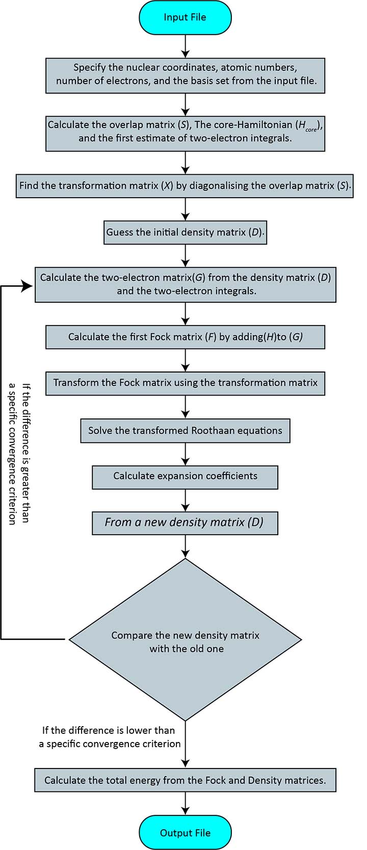
Let's break this down into a more detailed, step-by-step algorithm.

The SCF Algorithm Steps

1. Initialization:

   • Specify the molecular geometry (nuclear coordinates) and the total number of electrons.
   • Choose a basis set $\{{\varphi }_{\mu }\}$.
   • Calculate all the integrals that do not change during the iterations:
     • Overlap integrals: $S_{\mu \nu }$
     • One-electron integrals (kinetic energy $T_{\mu \nu }$ and nuclear attraction $V_{\mu \nu }$). These are combined to form the core Hamiltonian matrix: ${\mathbf{H}}^{\text{core}}=\mathbf{T}+\mathbf{V}$.
     • Two-electron integrals: $(\mu \nu |\lambda \sigma )$. These are the most numerous and computationally expensive integrals.

2. Orthogonalization:

   • The generalized eigenvalue problem $\mathbf{FC}=\mathbf{SCE}$ is inconvenient. We transform it into a standard eigenvalue problem by finding a transformation matrix $\mathbf{X}$ that makes the basis orthonormal. A common method is symmetric orthogonalization, where $\mathbf{X}={\mathbf{S}}^{-1/2}$.
   • This allows us to work with a transformed Fock matrix ${\mathbf{F}}^{\prime }={\mathbf{X}}^{†}\mathbf{FX}$ and solve the standard eigenvalue equation ${\mathbf{F}}^{\prime }{\mathbf{C}}^{\prime }={\mathbf{C}}^{\prime }\mathbf{E}$.

3. Initial Guess:

   • Make an initial guess for the coefficient matrix $\mathbf{C}$ (and thus the density matrix $\mathbf{P}$). A very simple guess is to assume the electrons feel no repulsion from each other initially. This is equivalent to setting $\mathbf{P}=0$, which makes the initial Fock matrix equal to the core Hamiltonian: ${\mathbf{F}}^{(0)}={\mathbf{H}}^{\text{core}}$.

4. SCF Iteration Loop:

   • (a) Build Fock Matrix: Using the current density matrix $\mathbf{P}$, construct the two-electron part of the Fock matrix, $\mathbf{G}$. The full Fock matrix for the current iteration $n$ is ${\mathbf{F}}^{(n)}={\mathbf{H}}^{\text{core}}+\mathbf{G}({\mathbf{P}}^{(n-1)})$.
   • (b) Solve Roothaan-Hall Equations:
     • Transform to the orthogonal basis: ${\mathbf{F}}^{\prime }={\mathbf{X}}^{†}{\mathbf{F}}^{(n)}\mathbf{X}$.
     • Diagonalize ${\mathbf{F}}^{\prime }$ to find the new orbital energies ${\mathbf{E}}^{(n)}$ and transformed coefficients ${{\mathbf{C}}^{\prime }}^{(n)}$.
     • Back-transform the coefficients to the original basis: ${\mathbf{C}}^{(n)}=\mathbf{X}{{\mathbf{C}}^{\prime }}^{(n)}$.
   • (c) Form New Density Matrix: Construct a new density matrix ${\mathbf{P}}^{(n)}$ using the coefficients ${\mathbf{C}}^{(n)}$ of the occupied molecular orbitals (determined by filling the orbitals from the lowest energy up, following the Aufbau principle). For a closed-shell system with $N$ electrons:
     $P_{\mu \nu }=2{\sum }_{i=1}^{N/2}{C}_{\mu i}^{\ast }{C}_{\nu i}$
   • (d) Check for Convergence: Compare the new density matrix ${\mathbf{P}}^{(n)}$ with the previous one ${\mathbf{P}}^{(n-1)}$, or compare the total energy from the current step with the previous one. If the difference is below a predefined threshold, the field is "self-consistent." The calculation is complete. If not, return to step (a) with the new density matrix ${\mathbf{P}}^{(n)}$.

The following video provides an excellent and detailed walkthrough of this entire algorithmic procedure.

3. From Algorithm to Code

Your background in physics and programming makes it valuable to see how this algorithm translates directly into code. You don't need to write a program from scratch, but understanding the structure of a simple HF code can solidify these concepts immensely.

The following resource provides a step-by-step guide to building a minimal Hartree-Fock program in Python using numpy. It's a perfect illustration of the SCF procedure in action.

This hands-on perspective demystifies the process, showing that at its core, the SCF procedure is a series of well-defined matrix manipulations, ideally suited for a computational approach.

Conclusion

In this lesson, we have mapped out the Self-Consistent Field (SCF) procedure, the workhorse algorithm for solving the Hartree-Fock equations.

Key Takeaways:

• The integro-differential HF equations are converted into the matrix-based Roothaan-Hall equations ($\mathbf{FC}=\mathbf{SCE}$) by introducing a basis set.
• The fact that the Fock matrix $\mathbf{F}$ depends on its own solutions ($\mathbf{C}$) necessitates an iterative solution.
• The SCF procedure follows a clear loop:
  1. Start with a guess for the electron density ($\mathbf{P}$).
  2. Build the Fock matrix $\mathbf{F}$.
  3. Solve the Roothaan-Hall equations (often after an orthogonalization step) to get new coefficients $\mathbf{C}$.
  4. Update the density matrix $\mathbf{P}$ using the new coefficients.
  5. Check for convergence. If not converged, repeat from step 2.
• This entire algorithm is fundamentally a sequence of matrix operations, making it highly suitable for computer implementation.

Preview of the Next Lesson:

The Hartree-Fock method, for all its power, is still an approximation. It treats each electron as moving in the average field of all others, but it neglects the instantaneous correlations in their motion, especially between electrons of opposite spin. The energy that the Hartree-Fock method fails to capture is known as the correlation energy. In our next lesson, we will formally define this crucial concept and discuss its physical significance, which will serve as our entry point into more advanced and accurate many-body theories.