DMFT Spectral Functions: Metals, Correlated Metals, and Mott Insulators

Recommended resources

The freely available resources this lesson will direct you to.

Hello! Welcome back to our course.

In the last lesson, we constructed the sophisticated machinery of Dynamical Mean-Field Theory. We saw how it maps an intractable many-body lattice problem onto a solvable quantum impurity model embedded in a self-consistent effective medium. We finished by outlining the iterative loop that, once converged, yields the local electronic Green's function, $G_{l oc} (ω)$ .

Today, we will reap the rewards of that theoretical effort. Our goal is to interpret the physical information contained within $G_{l oc} (ω)$ . We will connect it to the single-particle spectral function, a quantity directly accessible in experiments like photoemission spectroscopy, with which you have practical experience. By learning to read the spectral function, you will be able to distinguish between a simple metal, a Mott insulator, and the uniquely interesting state that lies between them: the strongly correlated metal. This lesson bridges the abstract theory of DMFT with the concrete, observable physics of strongly correlated materials.

1. The Spectral Function: What DMFT Calculates

The central output of the DMFT loop is the local Green's function, $G_{l oc} (ω)$ . Its imaginary part, with the proper normalization, gives us the local spectral function, often denoted $A (ω)$ or $ρ (ω)$ :

A (ω) = - \frac{1}{π} Im G_{l oc} (ω + i η)

where $η$ is an infinitesimal positive number. The spectral function has a profound physical meaning:

For $ω > E_{F}$ , $A (ω)$ is the probability density for adding an electron with energy $ω$ . This is probed experimentally by techniques like inverse photoemission spectroscopy (IPES) or X-ray absorption spectroscopy (XAS).
For $ω < E_{F}$ , $A (ω)$ is the probability density for removing an electron with energy $ω$ . This is what is measured in photoemission spectroscopy (PES).

Essentially, $A (ω)$ represents the density of available electronic states. A finite value of $A (ω)$ at the Fermi energy ( $ω = 0$ , by convention) signals a metal, while a vanishing value signifies a gap, characteristic of an insulator or semiconductor.

Our focus will be on the half-filled single-band Hubbard model, where the competition between kinetic energy (hopping $t$ or bandwidth $W$ ) and on-site Coulomb repulsion $U$ drives the Mott transition. We will analyze how $A (ω)$ evolves as we increase the ratio $U / W$ .

2. Evolution of the Spectral Function across the Mott Transition

The transition from a metal to a Mott insulator is not abrupt. DMFT reveals a rich evolution of the electronic states, which we can categorize into three main regimes. The following reading and figures will guide our discussion.

Dynamical mean-field theory for correlated electrons

The review article 'Dynamical mean-field theory for correlated electrons' by Dieter Vollhardt provides an excellent and clear description of how the spectral function evolves across the Mott transition. We will focus on the section describing this evolution.

Please read Section 4.1, 'DMFT and the three-peak structure of the spectral function' (page 9). Pay close attention to the schematic in Figure 5 and the corresponding numerical results in Figure 6. Try to map the features in the figures to the description in the text.

Let's break down the evolution shown in the reading.

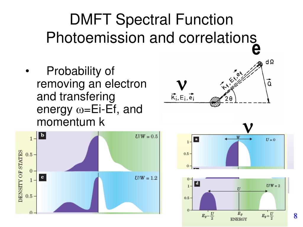
Case A: The Weakly Correlated Metal ( $U / W ≪ 1$ )

When the interaction $U$ is zero or very small compared to the bandwidth $W$ , the system behaves as predicted by standard band theory.

The spectral function $A (ω)$ simply reflects the non-interacting density of states (DOS). For the Bethe lattice often used in DMFT calculations, this is a semi-ellipse.
The system is a metal, with a large density of states at the Fermi energy ( $A (ω = 0) > 0$ ).
The electrons are well-described as itinerant Bloch waves, forming a Fermi liquid with long-lived quasiparticle excitations.

DMFT Spectral Function, Photoemission, and Correlations — This figure illustrates the evolution of the density of states (spectral function) with increasing interaction strength U/W. Panel (a) shows the non-interacting case (U=0), which corresponds to our weakly correlated metal. As we will see, panels (b), (c), and (d) represent the transition to a correlated metal and then a Mott insulator.

Case B: The Strongly Correlated Metal ( $U / W \sim 1$ )

This is where the physics becomes fascinating and deviates strongly from simple band theory. As $U$ becomes comparable to $W$ , the spectral function develops a characteristic three-peak structure:

Quasiparticle (QP) Peak: A sharp, coherent peak remains at the Fermi energy ( $ω = 0$ ). This peak represents the fraction of electrons that can still propagate through the lattice as itinerant, albeit heavy, quasiparticles. Its spectral weight, known as the quasiparticle residue $Z$ , is significantly reduced ( $Z < 1$ ). The effective mass of these quasiparticles is enhanced, $m^{*} = m / Z$ . The width of this peak is tied to a new, low-energy scale that is dynamically generated by correlations.
Lower and Upper Hubbard Bands (LHB & UHB): On either side of the QP peak, two broad, incoherent humps appear, centered roughly at $ω \approx - U /2$ and $ω \approx + U /2$ . These are the Hubbard bands. They represent high-energy, atomic-like excitations.
- The LHB corresponds to removing an electron from a singly occupied site.
- The UHB corresponds to adding an electron to a singly occupied site, creating a doubly-occupied site at an energy cost of $U$ .

This coexistence of a coherent quasiparticle peak with incoherent Hubbard bands is a hallmark of a strongly correlated metal. It reveals the dual nature of electrons in this regime: they simultaneously exhibit both wave-like (itinerant QP peak) and particle-like (localized Hubbard bands) character.

Case C: The Mott Insulator ( $U / W > U_{c 2} / W$ )

When the interaction $U$ exceeds a critical value $U_{c 2}$ , a dramatic change occurs:

The central quasiparticle peak completely vanishes ( $Z \to 0$ ).
The spectral function now consists only of the LHB and UHB, which are now fully separated.
A Mott-Hubbard gap opens up around the Fermi energy. Since $A (ω = 0) = 0$ , there are no available states for low-energy excitations.

The system has become a Mott insulator. This is not due to band filling (the band is still half-full) but purely due to the strong Coulomb repulsion, which localizes electrons on individual atomic sites to prevent costly double occupancy.

The resource below offers another perspective on this evolution, including how these features disperse with momentum, which is what an experiment like Angle-Resolved Photoemission Spectroscopy (ARPES) would measure.

Dynamical Mean-Field Theory and the Mott Transition

The document 'Dynamical Mean-Field Theory and the Mott Transition' by Marcelo Rozenberg provides a detailed analysis of the transition, including momentum-resolved spectral functions.

Please read Section 3.2 'The Mott-Hubbard transition' and Section 3.3 'Band-structure evolution across the metal-insulator transition' (pages 18-21). Focus on Figure 9, which shows the evolution of the DOS, and Figure 10, which shows the corresponding momentum-resolved spectral function A(ε, ω). Note how the coherent quasiparticle band in the metal is much flatter (heavier mass) than the non-interacting one.

Test your understanding!

Imagine you perform a photoemission spectroscopy (PES) experiment on a strongly correlated metal. Sketch the expected spectrum (intensity vs. binding energy) and label the features you would observe. Remember that PES only probes occupied states ( $ω < 0$ ).

Show answer

Your sketch should show PES intensity on the y-axis and binding energy on the x-axis (with $E = 0$ being the Fermi level and binding energy increasing to the left).

The spectrum should have two main features:

A sharp quasiparticle peak right at the Fermi energy ( $E = 0$ ).
A broad hump at a higher binding energy (e.g., around $E \approx U /2$ ). This is the Lower Hubbard Band (LHB).

The UHB would not be visible as it corresponds to unoccupied states. The presence of both features is the key signature of a correlated metal in PES.

3. Connecting Theory with Experiment

The three-peak spectral structure is not just a theoretical curiosity; it is directly observed in real materials. Your own experience with photoluminescence spectroscopy gives you an appreciation for how spectral features relate to electronic transitions. Photoemission is a very direct probe of the spectral function.

The image below beautifully illustrates this connection. It places PES data from several real transition metal oxides alongside the theoretical evolution of the DMFT spectral function.

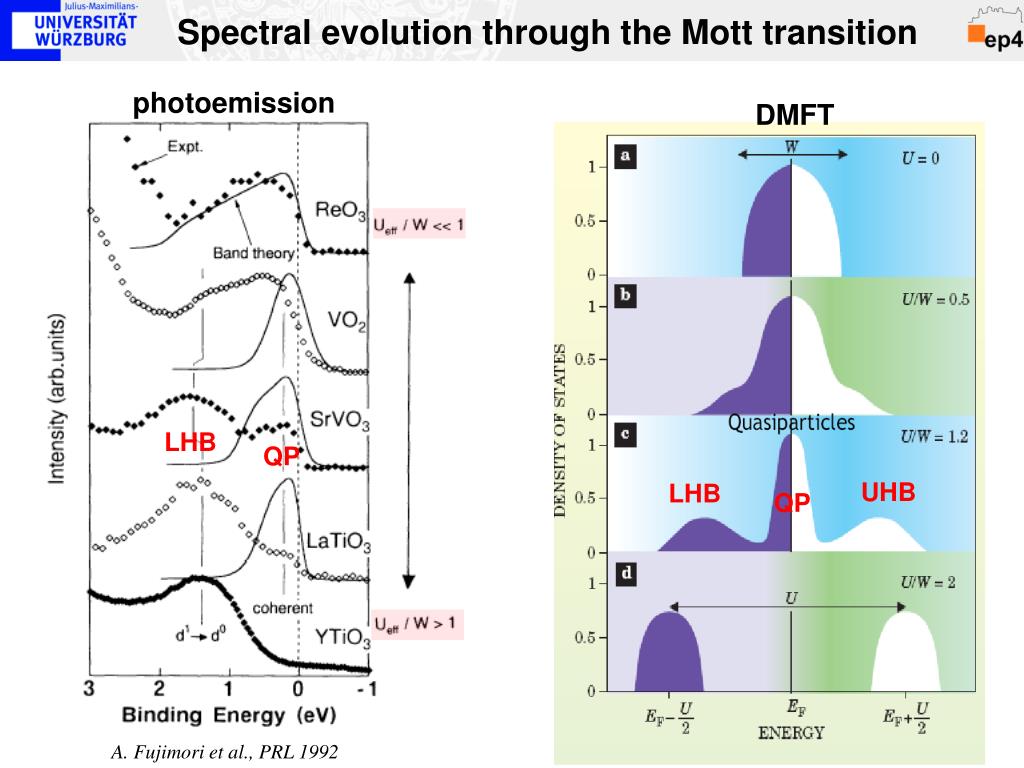
Spectral Evolution Through the Mott Transition: Photoemission and DMFT — A comparison of experimental photoemission spectra for various transition metal oxides (left) and theoretical DMFT spectral functions (right) as a function of increasing correlation strength U/W. The experimental data for materials like SrVO₃ clearly show the quasiparticle (QP) peak at the Fermi level and the Lower Hubbard Band (LHB), matching the DMFT prediction for a correlated metal. Materials like YTiO₃, which are more strongly correlated, show a suppressed QP peak and a prominent LHB, indicating they are on the verge of becoming or are already Mott insulators.

As shown in the figure, a material like SrVO₃ is a canonical example of a correlated metal. Its spectrum clearly exhibits both the quasiparticle peak at $E_{F}$ and the lower Hubbard band around -1.5 eV. In contrast, YTiO₃, with stronger effective correlations, shows a much-suppressed QP peak and is considered a Mott insulator. The remarkable agreement between the DMFT calculations and the experimental data was a major triumph for the theory, confirming that it correctly captures the essential physics of electron correlation.

Conclusion

In this lesson, we have learned how to decode the primary output of a DMFT calculation—the spectral function. By analyzing its shape, we can identify the physical state of a correlated electron system.

Key Takeaways:

The spectral function $A (ω) = - \frac{1}{π} Im G_{l oc} (ω)$ represents the density of available electronic states and is directly measured in photoemission experiments.
A weakly correlated metal shows a single broad band, similar to the non-interacting DOS.
A strongly correlated metal is characterized by a three-peak structure: a sharp, coherent quasiparticle peak at the Fermi level, flanked by broad, incoherent upper and lower Hubbard bands.
A Mott insulator exhibits a gap at the Fermi energy, with the spectral function consisting only of separated lower and upper Hubbard bands.

You are now equipped not only to understand the theoretical formulation of DMFT (from the previous lesson) but also to interpret its physical predictions and connect them to experimental reality.

Preview of the Next Lesson

We have just interpreted the spectral function based on the results from DMFT. In the next module, we will step back slightly to build a more general and formal foundation for many-body theory. The first lesson will be to derive the Lehmann representation of the Green's function. This powerful formalism provides a rigorous definition of the spectral function and formally proves its connection to the elementary excitations (quasiparticles) of a many-body system, providing a deeper justification for the interpretations we have used today.