Data Splitting: Train, Validate, and Test

Welcome to the first lesson in our module on model evaluation. In our last discussion, we explored polynomial regression and saw firsthand how increasing model complexity can lead to overfitting. We observed that a model with a very high degree could achieve near-perfect error on the data it was trained on, but performed poorly on new, unseen data. This raises a critical question: if training error is a misleading indicator of a model's true performance, how can we reliably estimate its ability to generalize?

This lesson addresses that question directly. We will explain the train/validation/test split methodology, which is the foundational practice for assessing and comparing machine learning models. Our goal is to understand the distinct role of each data subset and why this rigorous separation is absolutely essential for obtaining an unbiased estimate of a model's future performance.

The Cardinal Sin: Evaluating on Training Data

In the previous lesson, we saw that a high-degree polynomial could perfectly fit the training points. If we were to judge the model based on its error on that same data, we would be fooled into thinking we had an excellent model. This flawed approach is known as resubstitution validation.

The fundamental problem is that a model's performance on data it has already seen gives no information about its ability to generalize. A high-capacity model can simply "memorize" the training data, including its noise, rather than learning the true underlying pattern.

The paper "Model Evaluation, Model Selection, and Algorithm Selection in Machine Learning" by Sebastian Raschka provides a concise explanation of this pitfall.

The difference between the training error and the error on new data is often called the "optimism bias," and our goal is to get a realistic estimate of the latter. To do this, we must evaluate our model on data it has not been trained on.

The First Step: A Simple Train/Test Split

The most basic solution is the holdout method, where we partition our data into two distinct sets:

1. Training Set: The subset of data the model uses to learn its parameters. For example, in linear regression, this is the data used to calculate the optimal coefficient values (${\beta }_i$).
2. Test Set: A subset of data that is "held out" during training. It is used only at the very end to evaluate the final model's performance on unseen data.

This process provides a much more honest assessment of generalization error. However, as we will see, this two-way split is not sufficient when we need to tune our model.

The Pitfall of Hyperparameter Tuning

Let's return to our polynomial regression example. The degree of the polynomial, $p$, is not a parameter learned from the data; it's a hyperparameter—a configuration choice we must make before training begins. Other examples include the regularization strength $\lambda$ or the number of neighbors in a k-NN algorithm.

How do we choose the best value for $p$? A natural impulse might be to try several values (e.g., $p=1,2,...,10$), train a model for each, evaluate their performance on the test set, and pick the $p$ that gives the lowest test error.

This is a trap.

By using the test set to compare models and select the best hyperparameter, we are implicitly fitting our hyperparameters to the test set. Information from the test set has "leaked" into our model selection process. Consequently, the test set is no longer a truly independent measure of generalization performance. The performance estimate we get from it will be optimistically biased because we've chosen the model that works best on that specific test set.

Stanford's Andrew Ng provides a clear conceptual explanation of this critical issue in his CS229 lecture.

The Standard Solution: Train/Validation/Test Split

To solve the problem of data leakage while tuning hyperparameters, we introduce a third partition, the validation set (often called the development or "dev" set). This leads to the standard three-way data split methodology.

The roles are now clearly defined and strictly enforced:

1. Training Set: Used exclusively to fit the model's parameters (e.g., the weights of a neural network or the coefficients of a linear model). The model learns from this data.
2. Validation (or Dev) Set: Used to make modeling decisions. This includes tuning hyperparameters (like the polynomial degree $p$), comparing different types of models (e.g., SVM vs. Random Forest), or deciding on feature engineering strategies. You evaluate the models trained on the training set against the validation set and select the one that performs best.
3. Test (or Holdout) Set: Used only once at the very end of your project. After you have used the validation set to select your single best model, you evaluate its performance on the test set to get a final, unbiased estimate of its generalization error. This result is what you would report to stakeholders or in a research paper.

The following resource provides a detailed, step-by-step walkthrough of this three-way holdout method.

To see this process demonstrated in a more practical, code-oriented context, the following video walks through training, comparing models on a validation set, and reporting final performance on a holdout set.

Practical Considerations: Split Ratios and Bias

A common question is how to decide the size of each split.

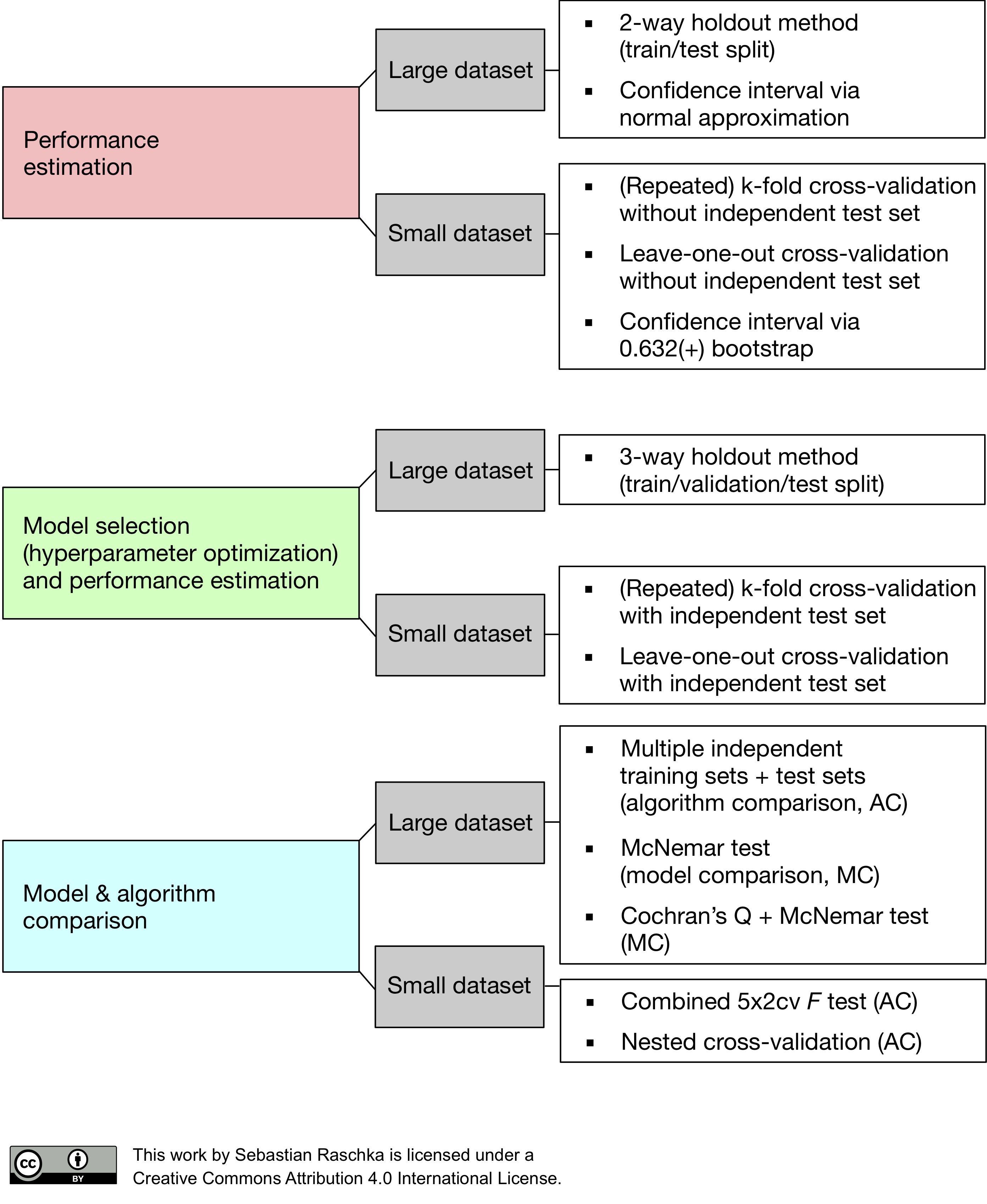
• Traditional Rule of Thumb: For small to medium datasets (hundreds to tens of thousands of examples), common splits are 70/30 (train/test) or 60/20/20 (train/validation/test).
• Modern Era of Big Data: When you have millions or billions of examples, the validation and test sets don't need to be proportionally large. Their purpose is to provide a statistically significant estimate of performance. For a dataset with 10 million examples, you might only need 100,000 for validation and 100,000 for testing. This allows you to use the vast majority of your data (e.g., 98% or 99%) for training, leading to a better model. The split might look more like 98/1/1.

It is also important to acknowledge a subtle trade-off. By withholding data for validation and testing, our training set is smaller than the total available data. A model trained on less data may perform slightly worse than a model trained on all the data. This can lead to a pessimistic bias in our performance estimate—we might be slightly underestimating the true performance of the final model that we could deploy (which would ideally be trained on all available data). This is an unavoidable consequence of needing a reliable evaluation protocol.

Conclusion

In this lesson, we have established the train/validation/test split as a cornerstone of rigorous machine learning practice. Its primary purpose is to provide an unbiased estimate of a model's ability to generalize to new, unseen data, preventing the self-deception that comes from evaluating a model on data it has already seen.

Key Takeaways:

• Train Set: Used to fit model parameters.
• Validation Set: Used to tune hyperparameters and perform model selection. This is the "development" phase.
• Test Set: A hermetically sealed dataset used only once at the end to report the final, unbiased performance of the selected model.
• This three-way split prevents information leakage from the test set into the model development process, which would otherwise lead to an overly optimistic performance estimate.
• Split ratios depend on dataset size; for very large datasets, the validation and test sets can be a much smaller percentage of the total data.

The train and validation sets are not just for evaluation; they are also powerful diagnostic tools. In our next lesson, we will explore how to use them to generate learning curves. By plotting model performance on the training and validation sets as a function of training data size, we can visually diagnose whether our model is suffering from high bias (underfitting) or high variance (overfitting), guiding our next steps in the model development cycle.