Discrete vs. Continuous Random Variables & Their Distributions

Introduction

In our last lesson, we built the foundation of probability theory from its axioms, learning to reason about abstract events like "a coin lands heads" or "a person has a disease." This framework is powerful, but in machine learning and computer graphics, we almost always work with numbers: pixel intensities, 3D coordinates, model parameters, or classification scores. This lesson introduces the crucial bridge between the abstract world of events and the numerical world of data: the random variable.

Our goal is to formally define random variables and explore the two fundamental types you will constantly encounter: discrete and continuous. We will introduce the specific mathematical tools used to describe each one: the Probability Mass Function (PMF) for discrete variables and the Probability Density Function (PDF) for continuous variables. Understanding this distinction is essential, as it dictates whether we use sums or integrals, a theme that will recur throughout your study of AI.

What is a Random Variable?

In the previous lesson, we defined an event as a subset of the sample space $\Omega$. A random variable is simply a function that assigns a specific numerical value to every possible outcome in that sample space.

Formally, a random variable $X$ is a function $X:\Omega \to \mathbb{R}$ that maps each outcome $\omega \in \Omega$ to a real number.

Let's make this concrete. Consider an experiment of flipping two coins. The sample space is $\Omega =\{HH,HT,TH,TT\}$. We can define a random variable $X$ to be the number of heads in the outcome:

• $X(HH)=2$
• $X(HT)=1$
• $X(TH)=1$
• $X(TT)=0$

This mapping allows us to rephrase questions about abstract events in numerical terms. The event "we get exactly one head" is formally the set of outcomes $\{HT,TH\}$. Using our random variable, we can express this same event as "$X=1$". This shorthand, "$X=x$", represents the event $\{\omega \in \Omega \mid X(\omega )=x\}$, which is the set of all outcomes that the random variable $X$ maps to the value $x$.

Professor Blitzstein provides a clear, intuitive explanation of this concept in his "pebble world" analogy.

The concept of a random variable naturally leads to a critical distinction. In our coin-flipping example, the number of heads can only be 0, 1, or 2. What if our random variable represented something like the exact temperature in a room? That value could be 20.1, 20.11, or 20.11034... It can take on any value within a continuous range. This brings us to the two main classes of random variables.

Discrete Random Variables and the Probability Mass Function (PMF)

A random variable is discrete if it can only take on a finite or countably infinite set of values. The number of heads in a coin toss, the result of a die roll, or the number of bugs in a piece of code are all examples of discrete random variables.

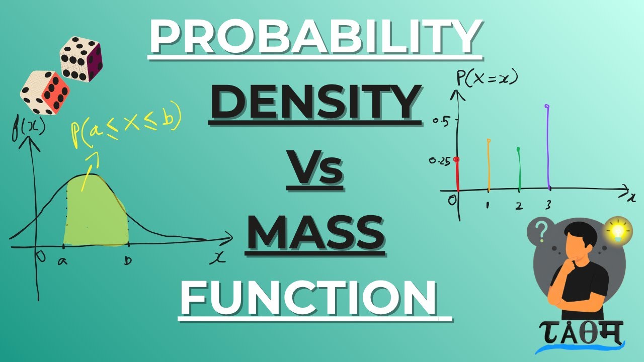
To describe the probabilistic behavior of a discrete random variable, we use a Probability Mass Function (PMF). The PMF, denoted $p_X(x)$, gives the probability that the random variable $X$ is equal to a specific value $x$.

$$p_X(x)=P(X=x)$$

For our two-coin-flip example, assuming fair coins:

• $p_X(0)=P(X=0)=P(\{TT\})=1/4$
• $p_X(1)=P(X=1)=P(\{HT,TH\})=2/4=1/2$
• $p_X(2)=P(X=2)=P(\{HH\})=1/4$
• $p_X(x)=0$ for all other values of $x$.

A valid PMF must satisfy two conditions:

1. Non-negativity: $p_X(x)\ge 0$ for all $x$.
2. Normalization: The sum of the probabilities over all possible values must be 1. ${\sum }_x{p}_X(x)=1$.

The following video provides a more detailed explanation of discrete random variables and their PMFs.

Continuous Random Variables and the Probability Density Function (PDF)

Now, let's consider a random variable that can take any value in an interval, like the exact position of a particle or the amount of rainfall. This is a continuous random variable.

Here we face a puzzle. If a variable can take on an infinite number of values, what is the probability of it taking on any single exact value? For example, if we spin a wheel of fortune with a perfectly precise pointer that can land anywhere between 0 and 1, what is the probability it lands on exactly 0.5?

The probability of hitting any single, infinitely precise point is zero. If it were non-zero, and we summed the probabilities of all the infinite points, the total would be infinite, violating the axiom that total probability must be 1. This means the PMF is not a useful tool for continuous variables, since $P(X=x)=0$ for all $x$.

Instead, we use a Probability Density Function (PDF), denoted $f_X(x)$. The PDF has a different interpretation than the PMF. The value of the PDF at a point $x$, $f_X(x)$, is not a probability. It is a measure of probability density around that point. It tells you how likely it is that the random variable will fall into a tiny interval around $x$.

For a continuous random variable, we find the probability of it falling within a range $[a,b]$ by calculating the area under the PDF curve over that interval. This is done using an integral:

$$P(a\le X\le b)={\int }_a^b{f}_X(x)dx$$

A valid PDF must satisfy two analogous conditions to the PMF:

1. Non-negativity: $f_X(x)\ge 0$ for all $x$.
2. Normalization: The total area under the curve must be 1. ${\int }_{-\infty }^{\infty }{f}_X(x)dx=1$.

The following video from MIT OpenCourseWare provides an excellent introduction to this concept.

To reinforce these ideas with text, the following reading provides concise, formal definitions.

The Cumulative Distribution Function (CDF): A Unifying View

While PMFs and PDFs are specific to discrete and continuous variables, respectively, the Cumulative Distribution Function (CDF) is a universal tool that applies to both. The CDF, denoted $F_X(x)$, is defined as the probability that the random variable $X$ takes on a value less than or equal to $x$.

$$F_X(x)=P(X\le x)$$

• For a discrete variable, the CDF is found by summing the PMF: $F_X(x)={\sum }_{x_i\le x}{p}_X(x_i)$. This results in a "staircase" function that jumps at each possible value.
• For a continuous variable, the CDF is found by integrating the PDF: $F_X(x)={\int }_{-\infty }^x{f}_X(t)dt$. This results in a smooth, non-decreasing function.

This relationship also gives us a powerful connection from calculus: for a continuous random variable, the PDF is the derivative of the CDF.

$$f_X(x)=\frac{d}{dx}{F}_X(x)$$

The CDF is a cornerstone of probabilistic modeling and is especially important in computer graphics for techniques like inverse transform sampling, which is used to generate random numbers that follow a specific distribution—a key step in rendering realistic scenes.

Conclusion

In this lesson, we made the critical transition from abstract events to numerical random variables. This allows us to apply the tools of calculus and algebra to the domain of probability, a necessary step for developing machine learning algorithms.

Key Takeaways:

• A random variable is a function that maps outcomes from a sample space to real numbers.
• Discrete random variables take on a countable set of values and are described by a Probability Mass Function (PMF), $p_X(x)=P(X=x)$, which gives the probability at each point. The PMF values sum to 1.
• Continuous random variables can take any value within an interval. They are described by a Probability Density Function (PDF), $f_X(x)$. Probabilities are calculated as the area (integral) under the PDF curve. The total area is 1.
• For a continuous variable, the probability of it taking any single exact value is zero.
• The Cumulative Distribution Function (CDF), $F_X(x)=P(X\le x)$, is a universal concept that gives the cumulative probability up to a value $x$, and it uniquely defines the distribution for any type of random variable.

Preview of the Next Lesson:
Now that we have functions (PMFs and PDFs) to describe the full behavior of a random variable, our next step is to learn how to summarize these distributions with a few key numbers. We will explore the concepts of expectation (mean) and variance. These are not just statistical curiosities; they are the fundamental building blocks for defining objective functions in optimization, measuring error in predictions, and understanding the stability of learning algorithms.