Probability Fundamentals

Introduction

Welcome to our first lesson on probability theory. In the previous modules, we built a robust toolkit from linear algebra and multivariable calculus, culminating in the ability to find and classify the extrema of complex functions. This was a journey through a deterministic world where functions and their properties were precisely known. Now, we pivot to the realm of uncertainty.

Machine learning and artificial intelligence are fundamentally about building models that can reason and make predictions from incomplete or noisy data. To do this, we need a formal language to quantify uncertainty, update our beliefs, and define the very objectives our optimization algorithms, like gradient descent, will target. That language is probability theory.

This lesson lays the groundwork. We will start from the 'first principles' of probability—the axioms that govern the entire field—and build up to the essential concepts of conditional, joint, and marginal probability. These rules form the grammar for reasoning under uncertainty, a skill that is indispensable for everything that follows, from understanding loss functions to developing advanced generative models.

The Axiomatic Foundation of Probability

Just as geometry is built on axioms about points and lines, probability theory is built on a simple set of rules governing sets and numbers. These rules, known as the Kolmogorov Axioms, provide a rigorous foundation for everything we will do. The core idea is to define a probability space, which consists of three components:

1. Sample Space ($\Omega$): The set of all possible outcomes of an experiment. For a single die roll, $\Omega =\{1,2,3,4,5,6\}$.
2. Event Space ($\mathcal{F}$): A collection of subsets of $\Omega$, which we call "events". An event is a set of outcomes we might be interested in. For a die roll, the event "the result is even" corresponds to the set $A=\{2,4,6\}$.
3. Probability Measure ($P$): A function that assigns a real number between 0 and 1 to every event in $\mathcal{F}$. $P(A)$ is the "probability of event A".

The following video from Harvard's Statistics 110 course, taught by Prof. Joseph Blitzstein (whose book you are reading), introduces this formal definition and the two essential axioms that the probability measure $P$ must satisfy.

To summarize and formalize what you just saw, the axioms are:

1. Non-negativity: For any event $A$, $P(A)\ge 0$.
2. Normalization: The probability of the entire sample space is 1, i.e., $P(\Omega )=1$. This means some outcome must occur.
3. Additivity: For any countable collection of pairwise disjoint events $A_1,A_2,\dots$ (meaning $A_i\cap A_j=\varnothing$ for $i\ne j$), the probability of their union is the sum of their individual probabilities: $$P\left(\bigcup _{i=1}^{\infty }{A}_i\right)=\sum _{i=1}^{\infty }P(A_i)$$

For a more formal and textual reinforcement of these ideas, you can review the following resource.

Now for your first challenge. Using only the three axioms above, can you prove that for any event $A$, its probability cannot exceed 1 (i.e., $P(A)\le 1$)? Hint: Consider the event $A$ and its complement, $A^c$. What is their relationship? What do you know about their union?

Joint, Conditional, and Marginal Probability

With the axioms in place, we can now define the key relationships between events that form the core of probabilistic reasoning.

Joint Probability

The joint probability of two events, $P(A\cap B)$ or $P(A,B)$, is simply the probability that both events occur. In a Venn diagram, this is the area of their intersection.

Conditional Probability

This is perhaps the most important concept in all of statistics. The conditional probability of $A$ given $B$, written $P(A|B)$, is the probability that event $A$ occurs, given that we know event $B$ has already occurred.

The definition is:

Intuitively, knowing that $B$ occurred restricts our sample space from the original $\Omega$ to just the outcomes in $B$. We then "renormalize" the probability of the part of $A$ that is also in $B$ (i.e., $A\cap B$) by the probability of this new, smaller universe, $P(B)$.

Prof. Blitzstein offers a fantastic philosophical motivation and two powerful intuitions for this definition.

Marginal Probability

The marginal probability is just the standard, "unconditional" probability of a single event, like $P(A)$. The term "marginal" comes from how it's calculated in a table of joint probabilities. To find the probability of one event, we sum over all possible outcomes of the other event. This is an application of the Law of Total Probability. If a set of events $B_1,B_2,\dots ,B_n$ forms a partition of the sample space (they are disjoint and their union is $\Omega$), then:

Using the definition of conditional probability, this becomes the more common form:

The image below provides a perfect visualization for these three concepts in a discrete setting. The numbers in the center of the table are the joint probabilities. The numbers in the margins are the marginal probabilities, obtained by summing the rows or columns. A conditional probability could be found by, for example, dividing a joint probability by a marginal probability (e.g., $P(\text{Maths}|\text{Male})=P(\text{Maths, Male})/P(\text{Male})=0.4/0.5=0.8$).

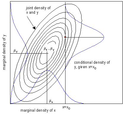
For continuous variables, the same concepts apply, but summation is replaced by integration. The image below provides the continuous analog. The contours represent the joint probability density. Slicing the distribution vertically gives a conditional density (the bell curve labeled "conditional density of y, given x=x₀"). Projecting the distribution onto an axis gives a marginal density.

Independence

Two events $A$ and $B$ are independent if the occurrence of one does not affect the probability of the other. Formally, this means $P(A|B)=P(A)$. Plugging this into the definition of conditional probability gives us the standard test for independence:

It is critical not to confuse independent events with disjoint events. Disjoint events have no outcomes in common ($A\cap B=\varnothing$), so $P(A\cap B)=0$. If you know a disjoint event $B$ occurred (and $P(B)>0$), you know with certainty that $A$ did not occur. This makes them highly dependent.

The following resource provides clear definitions and examples to solidify these concepts.

The Multiplication Rule and Bayes' Rule

Two simple but powerful theorems follow directly from the definition of conditional probability.

1. The Multiplication Rule: By rearranging the definition $P(A|B)=P(A\cap B)/P(B)$, we get a formula for the joint probability:

   $$P(A\cap B)=P(A|B)P(B)$$

   By symmetry, it's also true that $P(A\cap B)=P(B|A)P(A)$. This rule is essential for calculating the probability of a sequence of events.

2. Bayes' Rule: Since both expressions for the multiplication rule equal $P(A\cap B)$, we can set them equal to each other:

   $$P(A|B)P(B)=P(B|A)P(A)$$

   Dividing by $P(B)$ gives the famous Bayes' Rule:

   $$P(A|B)=\frac{P(B|A)P(A)}{P(B)}$$

   This rule is the engine of Bayesian statistics. It tells us how to "invert" our conditional probabilities—how to update our belief in event $A$ ($P(A|B)$) after observing event $B$, using our prior belief in $A$ ($P(A)$) and the likelihood of observing $B$ if $A$ were true ($P(B|A)$).

Prof. Blitzstein derives both of these rules very quickly in the final segment of the lecture.

Now for a classic problem that tests your understanding of these rules.

Imagine a test for a rare disease. Only 1 in 10,000 people have the disease. The test is very good, but not perfect.

• It correctly identifies 99% of people who have the disease (99% sensitivity).
• It correctly identifies 99% of people who do not have the disease (99% specificity). This means it has a 1% "false positive" rate.

A person is chosen at random and tests positive. Before you calculate, what is your intuition—is it almost certain they have the disease, a 50/50 chance, or something else? Now, use the rules we've learned to calculate the actual probability that this person has the disease, given they tested positive.

Conclusion

In this lesson, we established the formal language of probability. We started from the fundamental axioms and used them to define and explore the relationships between events. These concepts are not just abstract mathematical rules; they are the tools we use to model the world and update our knowledge in the face of new data.

Key Takeaways:

• Probability theory is built upon three simple axioms: non-negativity, normalization, and additivity for disjoint events.
• Joint Probability $P(A,B)$ is the probability of $A$ and $B$ both occurring.
• Conditional Probability $P(A|B)=P(A,B)/P(B)$ is the updated probability of $A$ given that $B$ is known to have occurred.
• Marginal Probability $P(A)$ is the overall probability of an event, which can be found by summing or integrating joint probabilities over all other events (the Law of Total Probability).
• Two events are independent if $P(A,B)=P(A)P(B)$, which implies $P(A|B)=P(A)$.
• Bayes' Rule, $P(A|B)=\frac{P(B|A)P(A)}{P(B)}$, provides a mechanism for inverting conditional probabilities and forms the basis of Bayesian inference.

Preview of the Next Lesson:
We will move from abstract events to random variables. A random variable is a function that assigns a numerical value to each outcome in the sample space. This is the crucial step that allows us to connect probability theory to the numerical data used in machine learning. We will explore how to describe the behavior of discrete random variables with Probability Mass Functions (PMFs) and continuous random variables with Probability Density Functions (PDFs).