Dot Product: Calculation and Geometric Meaning

In our previous lesson, we established the foundational concept of a vector, understanding it dually as a geometric arrow and a numerical list of coordinates. We saw how the simple operations of addition and scalar multiplication allow us to navigate and scale these vectors. Now, we will introduce a new kind of vector multiplication, one that will unlock a much richer geometric understanding of the spaces these vectors inhabit.

This lesson focuses on the dot product, also known as the scalar product. You will learn not only how to compute it but, more critically, what the resulting scalar value tells us about the relationship between two vectors. This single operation is the key to measuring angles, determining orthogonality (perpendicularity), and calculating projections—concepts that are indispensable in fields from computer graphics lighting models to machine learning similarity metrics.

Defining the Dot Product

We will begin with the most direct way to compute the dot product, which arises from the coordinate representation of vectors.

For two vectors $\mathbf{a}$ and $\mathbf{b}$ in ${\mathbb{R}}^n$, their dot product, denoted $\mathbf{a}\cdot \mathbf{b}$, is found by multiplying their corresponding components and summing the results.

$$\mathbf{a}\cdot \mathbf{b}=\sum _{i=1}^n{a}_i{b}_i=a_1{b}_1+a_2{b}_2+\cdots +a_n{b}_n$$

For instance, if $\mathbf{a}=\left[\begin{array}{c}1\\ 2\\ 3\end{array}\right]$ and $\mathbf{b}=\left[\begin{array}{c}-2\\ 0\\ 4\end{array}\right]$, their dot product is:

$$\mathbf{a}\cdot \mathbf{b}=(1\times -2)+(2\times 0)+(3\times 4)=-2+0+12=10$$

Notice that the result is a single number—a scalar—not a vector. This is why it's often called the scalar product.

This calculation is straightforward, but its true power is hidden. This leads to a crucial question: What geometric information does this resulting scalar value encode? What is the fundamental difference between a dot product of 10, 0, or -5?

The Geometric Interpretation: Angle and Projection

The answer to our question lies in the geometric definition of the dot product, which is arguably the more fundamental one. It connects the dot product to the lengths (magnitudes) of the vectors and the angle between them.

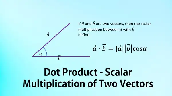
The geometric formula for the dot product is:

$$\mathbf{a}\cdot \mathbf{b}=|\mathbf{a}||\mathbf{b}|\cos (\theta )$$

Here, $|\mathbf{a}|$ and $|\mathbf{b}|$ are the magnitudes (or L2 norms) of the vectors, and $\theta$ is the angle between them when they are placed tail-to-tail.

This formula reveals everything. The dot product's sign and magnitude tell us about the vectors' relative alignment:

• $\mathbf{a}\cdot \mathbf{b}>0$: $\cos (\theta )>0$, so the angle $\theta$ is less than 90°. The vectors point in a generally similar direction.
• $\mathbf{a}\cdot \mathbf{b}=0$: $\cos (\theta )=0$, so the angle $\theta$ is exactly 90°. The vectors are orthogonal (perpendicular). This is one of the most important properties of the dot product.
• $\mathbf{a}\cdot \mathbf{b}<0$: $\cos (\theta )<0$, so the angle $\theta$ is greater than 90°. The vectors point in generally opposite directions.

The video below from Math and Science offers an excellent, detailed walkthrough of this geometric significance, introducing the powerful analogy of projection.

As the video explains, the dot product is fundamentally about projection. Think of the term $|\mathbf{b}|\cos (\theta )$. This is the length of the "shadow" that vector $\mathbf{b}$ casts onto vector $\mathbf{a}$. This "shadow" is the scalar projection of $\mathbf{b}$ onto $\mathbf{a}$.

So, the dot product $\mathbf{a}\cdot \mathbf{b}$ can be interpreted as:
(Length of $\mathbf{a}$) $\times$ (Scalar projection of $\mathbf{b}$ onto $\mathbf{a}$)

Symmetrically, it is also:
(Length of $\mathbf{b}$) $\times$ (Scalar projection of $\mathbf{a}$ onto $\mathbf{b}$)

This gives us the tools to formally define projection.

Given two vectors $\mathbf{a}$ and $\mathbf{b}$:

1. Scalar Projection of $\mathbf{a}$ onto $\mathbf{b}$ (the length of the shadow):

   $${\text{comp}}_{\mathbf{b}}(\mathbf{a})=|\mathbf{a}|\cos (\theta )=\frac{\mathbf{a}\cdot \mathbf{b}}{|\mathbf{b}|}$$

2. Vector Projection of $\mathbf{a}$ onto $\mathbf{b}$ (the shadow as a vector): We get this by taking the scalar projection (a length) and multiplying it by the unit vector in the direction of $\mathbf{b}$, which is $\frac{\mathbf{b}}{|\mathbf{b}|}$.

   $${\text{proj}}_{\mathbf{b}}(\mathbf{a})=\left(\frac{\mathbf{a}\cdot \mathbf{b}}{|\mathbf{b}|}\right)\frac{\mathbf{b}}{|\mathbf{b}|}=\left(\frac{\mathbf{a}\cdot \mathbf{b}}{|\mathbf{b}{|}^2}\right)\mathbf{b}=\left(\frac{\mathbf{a}\cdot \mathbf{b}}{\mathbf{b}\cdot \mathbf{b}}\right)\mathbf{b}$$

These projection formulas are cornerstones of many algorithms in graphics (like decomposing light reflection) and machine learning (like the Gram-Schmidt process).

Bridging the Definitions: A First-Principles Derivation

We now have two formulas for the same operation. A key tenet of a first-principles approach is understanding why these are equivalent. We can derive the algebraic formula from the geometric one.

Consider two vectors $\mathbf{v}$ and $\mathbf{w}$ in 2D. We can express them in terms of the standard basis vectors $\hat{i}=\left[\begin{array}{c}1\\ 0\end{array}\right]$ and $\hat{j}=\left[\begin{array}{c}0\\ 1\end{array}\right]$:

$$\mathbf{v}=v_x\hat{i}+v_y\hat{j}\text{and}\mathbf{w}=w_x\hat{i}+w_y\hat{j}$$

The dot product is distributive over addition (a property proven geometrically in the reading below). So we can write:

$$\mathbf{v}\cdot \mathbf{w}=(v_x\hat{i}+v_y\hat{j})\cdot (w_x\hat{i}+w_y\hat{j})$$ $$\mathbf{v}\cdot \mathbf{w}=v_x{w}_x(\hat{i}\cdot \hat{i})+v_x{w}_y(\hat{i}\cdot \hat{j})+v_y{w}_x(\hat{j}\cdot \hat{i})+v_y{w}_y(\hat{j}\cdot \hat{j})$$

Now, using only the geometric definition $\mathbf{a}\cdot \mathbf{b}=|\mathbf{a}||\mathbf{b}|\cos (\theta )$, what are the values of the dot products of the basis vectors?

• What is $\hat{i}\cdot \hat{i}$? (Hint: The angle of a vector with itself is 0°).
• What is $\hat{i}\cdot \hat{j}$? (Hint: The standard basis vectors are orthogonal).

You should find that $\hat{i}\cdot \hat{i}=|\hat{i}||\hat{i}|\cos (0^{\circ })=1\times 1\times 1=1$. Similarly, $\hat{j}\cdot \hat{j}=1$.
For the cross-term, $\hat{i}\cdot \hat{j}=|\hat{i}||\hat{j}|\cos (90^{\circ })=1\times 1\times 0=0$.

Substituting these back into our expanded equation, the two middle terms vanish:

$$\mathbf{v}\cdot \mathbf{w}=v_x{w}_x(1)+v_x{w}_y(0)+v_y{w}_x(0)+v_y{w}_y(1)$$ $$\mathbf{v}\cdot \mathbf{w}=v_x{w}_x+v_y{w}_y$$

This is precisely the algebraic formula we started with. This derivation shows that the component-wise formula is a direct consequence of the geometric behavior of an orthonormal basis.

The following short paper elegantly argues for this "geometry-first" approach.

Applications in Graphics and Machine Learning

With both definitions in hand, the dot product becomes a powerful and practical tool.

1. Finding the Angle Between Vectors: By rearranging the geometric formula, we can directly compute the angle between any two non-zero vectors:

   $$\theta =\arccos \left(\frac{\mathbf{a}\cdot \mathbf{b}}{|\mathbf{a}||\mathbf{b}|}\right)$$

   This is fundamental in graphics for everything from calculating how light reflects off a surface to determining if a polygon is facing the camera.

2. Measuring Similarity (Cosine Similarity): In machine learning, vectors can represent complex data like documents or images. Often, we care more about the "direction" (the content) of these vectors than their magnitude (e.g., document length). Cosine Similarity measures exactly this, and it is simply the cosine of the angle between the vectors:

   $$\text{Similarity}=\cos (\theta )=\frac{\mathbf{a}\cdot \mathbf{b}}{|\mathbf{a}||\mathbf{b}|}$$

   This value ranges from -1 (perfectly opposite) to 1 (perfectly aligned), providing a normalized score of how similar two vectors are.

To explore these applications and see how to implement them, the following resource is very helpful.

Conclusion

In this lesson, you have moved beyond simple vector arithmetic into the realm of geometric analysis. We have shown that the dot product is far more than a rote calculation; it is a profound tool that connects the algebraic and geometric worlds.

You learned that the dot product can be computed by summing the products of corresponding components, and that this simple operation has a deep geometric meaning: it measures the extent to which two vectors align. This interpretation gives us the tools to define orthogonality, calculate the angle between vectors, and compute the projection of one vector onto another. Finally, we saw how these capabilities translate directly into critical applications like cosine similarity in machine learning and lighting calculations in computer graphics.

In our next lesson, we will introduce the matrix. If vectors are the nouns of linear algebra, matrices are the verbs. You will learn to compute matrix-vector and matrix-matrix products and, crucially, to see matrices not just as tables of numbers, but as operators that perform geometric transformations—like rotations, scales, and shears—on vectors. The dot product's role in understanding projections and angles is a first step toward this deeper understanding of linear transformations.