Matrix Multiplication as Transformations

Recommended resources

The freely available resources this lesson will direct you to.

Welcome to our third lesson in the linear algebra module. In our previous discussions, we've built up an understanding of vectors as both geometric arrows and lists of numbers, and we explored how the dot product reveals the angular relationship between them. Now, we shift our focus from the objects themselves—vectors—to the actions we can perform on them.

This lesson introduces the matrix. You will learn to compute matrix-vector and matrix-matrix products, but more importantly, you will learn to see matrices for what they truly are: operators that encode geometric transformations. We will discover how actions like rotation, scaling, and shearing are captured in these grids of numbers. This perspective is the absolute cornerstone of computer graphics and a key concept in understanding how neural networks process data.

To begin, let's consider a simple geometric action: rotating every vector in a 2D plane by 90 degrees counter-clockwise. How would you go about describing this transformation using only numbers, such that a computer could apply it to any vector $[x y]$ ? What minimal set of numbers would you need to store?

From Geometric Action to Matrix-Vector Multiplication

The word "transformation" is essentially a synonym for "function," but used in linear algebra to evoke the idea of movement. A transformation takes an input vector and maps it to an output vector. We are interested in a special class called linear transformations.

Visually, a transformation is linear if it keeps space looking like a grid:

All lines in the grid must remain lines (they don't get curved).
The origin must remain fixed in place.

This implies that the grid lines remain parallel and evenly spaced after the transformation.

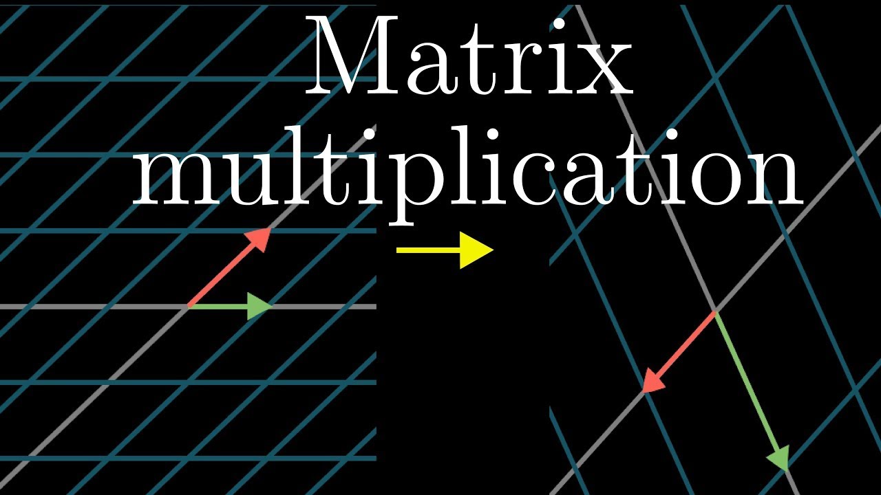
A linear transformation warps space, but grid lines remain parallel and evenly spaced.

The key insight, and the answer to our opening question, is that we don't need to describe what happens to every vector. We only need to record where the basis vectors land. In 2D, these are $i^= [10]$ and $j^= [01]$ .

Any vector $v = [x y]$ is just a linear combination of these basis vectors: $v = x i^+ y j^$ . Because a linear transformation preserves this "grid structure," the transformed vector, let's call it $L (v)$ , will be the same linear combination of the transformed basis vectors:

L (v) = x \cdot L (i^) + y \cdot L (j^)

This is a profound idea. The entire transformation is completely determined by just two vectors: where $i^$ goes and where $j^$ goes.

The following video from 3Blue1Brown provides an exceptional visualization of this concept.

Linear transformations and matrices | Chapter 3, Essence of linear algebra

This video, "Linear transformations and matrices," is a masterclass in building intuition for the connection between matrices and the transformation of space.

Please watch the first three segments. The first part, "Linear transformation," defines the concept visually. The second part, "Describing transformations with numbers," explains the crucial idea that a transformation is fully described by where the basis vectors land. The third part, "The 2x2 matrix," shows how we package this information into a matrix and how matrix-vector multiplication emerges naturally.

As the video explains, we package the coordinates of the transformed basis vectors into a matrix. The first column of the matrix is the vector where $i^$ lands, and the second column is where $j^$ lands.

If a transformation takes $i^$ to $[a c]$ and $j^$ to $[b d]$ , the matrix for this transformation is $M = [a c b d]$ .

Applying this transformation to a vector $v = [x y]$ is called matrix-vector multiplication. The calculation is precisely the linear combination we discussed:

Mv = [a c b d] [x y] = x [a c] + y [b d] = [a x + b y c x + d y]

This is the fundamental definition of matrix-vector multiplication. It is not just a random set of rules; it is the computational result of applying a geometric transformation.

For example, for a 90-degree counter-clockwise rotation:

$i^= [10]$ lands on $[01]$ .
$j^= [01]$ lands on $[- 1 0]$ .

The rotation matrix is therefore $R_{90} = [01 - 1 0]$ .

Composing Transformations: Matrix-Matrix Multiplication

What happens if we apply one transformation followed by another? For example, a rotation followed by a shear. The result of these two successive actions is itself a new, single linear transformation. This is called the composition of the two transformations.

How do we find the matrix for this composite transformation? We use the same logic as before: we just need to track where the basis vectors, $i^$ and $j^$ , end up after the entire sequence.

Suppose we apply transformation $A$ first, then transformation $B$ . The composite transformation is written as $BA$ (the order is right-to-left, just like function composition, e.g., $f (g (x))$ ).

Track $i^$ : After transformation $A$ , $i^$ becomes the first column of $A$ , let's call it $a_{1}$ . Now we apply transformation $B$ to this new vector. The final landing spot is $B a_{1}$ . This resulting vector becomes the first column of our new composite matrix.
Track $j^$ : Similarly, $j^$ first becomes the second column of $A$ ( $a_{2}$ ), and its final landing spot is $B a_{2}$ . This is the second column of the composite matrix.

Therefore, the product of two matrices $BA$ is the matrix whose columns are the result of applying transformation $B$ to each of the column vectors of $A$ .

The next video from 3Blue1Brown illustrates this beautifully.

Matrix multiplication as composition | Chapter 4, Essence of linear algebra

This video, "Matrix multiplication as composition," extends the geometric intuition to the product of two matrices.

Focus on these two key segments: "Composition of transformations" introduces the core idea that multiplying matrices is equivalent to composing their corresponding transformations. Pay attention to the right-to-left notation. "Numerical computation" walks through the symbolic derivation, showing how the columns of the product matrix are formed.

This geometric view is powerful. For a more formal textual summary of these ideas, the following blog post is an excellent read.

Matrix multiplication - Matthew N. Bernstein

This article clearly outlines different perspectives on matrix multiplication, emphasizing the composition of linear transformations as the most powerful one.

Start by reading the Introduction and Definition. Then, review the section that outlines the three perspectives, focusing on Perspective 1 and Perspective 3. You can read these sections starting from here.

The Computational Shortcut: Row-Column Rule

While the "transformation of columns" view provides the core intuition, there is a more common-day computational rule that you might have seen before. The element in the $i$ -th row and $j$ -th column of a product matrix $C = AB$ is the dot product of the $i$ -th row of $A$ and the $j$ -th column of $B$ .

This diagram shows the row-column rule. Each entry in the resulting matrix is a dot product of a row from the first matrix and a column from the second.

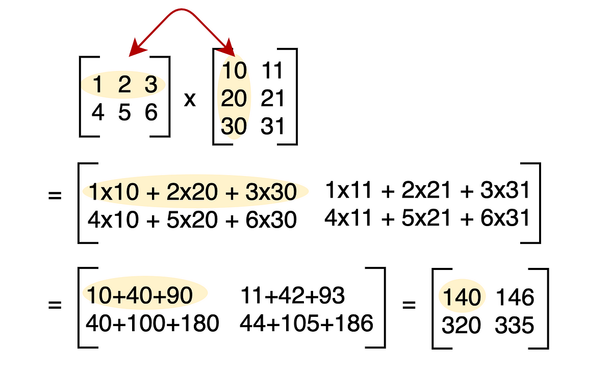
Let $A$ be an $m \times n$ matrix and $B$ be an $n \times p$ matrix. Their product $C = AB$ will be an $m \times p$ matrix, where the entry $C_{ij}$ is:

C_{ij} = (row i of A) \cdot (column j of B) = k = 1 \sum n A_{ik} B_{k j}

This rule seems arbitrary at first, but it is a direct consequence of the "linear combination of columns" definition we started with. It's simply a different way to organize the same arithmetic. This connection to the dot product from our last lesson is not a coincidence; it arises from the underlying geometric structure.

Properties and Consequences

Viewing matrix multiplication as a composition of transformations makes some of its properties very intuitive.

Non-Commutativity: In general, $AB \neq = BA$ . This is obvious geometrically. Rotating then shearing gives a different result than shearing then rotating. Order matters!
Associativity: $(AB) C = A (BC)$ . This property is also self-evident. Applying transformation C, then B, then A is the same sequence of actions regardless of how you group them.
Dimensionality: For a product $AB$ to be defined, the number of columns in $A$ must equal the number of rows in $B$ . From a transformation standpoint, this means the output dimension of the first transformation ( $B$ ) must match the input dimension of the second transformation ( $A$ ). For example, if $B$ maps 3D space to 2D space, $A$ must be a transformation that takes vectors from 2D space.

Conclusion

In this lesson, we have reframed matrices from static tables of numbers into dynamic operators that represent linear transformations. This is the "first principles" view that unlocks a deeper understanding of linear algebra.

We have established that:

A matrix's columns are the landing spots of the basis vectors under a linear transformation.
Matrix-vector multiplication is the computation that applies this transformation to a specific vector.
Matrix-matrix multiplication corresponds to the composition of two linear transformations, and its columns can be found by transforming the columns of the right-hand matrix.
The familiar row-column rule for computation is simply a compact way to perform the arithmetic derived from these geometric foundations.

In our next lesson, we will transition from theory to practice. You will implement matrix-vector and matrix-matrix multiplication from scratch. This exercise will not only solidify your understanding of the mechanics but also serve as the first practical step toward building the computational engines for computer graphics and neural networks.