Recommended resources
The freely available resources this lesson will direct you to.
Hello. Last lesson, you chose evaluation measures by asking what false positives and false negatives cost. Now you can put those measures to work: is a learned model actually better than a straightforward alternative? This final lesson in the foundations module shows how to choose, build, and fairly evaluate a baseline. Allow about 35–40 minutes, including the short videos and reading.
A baseline makes “better” meaningful
Suppose a fraud model catches 80% of fraudulent transactions. That sounds promising, but it leaves an important question unanswered: what would happen if you simply followed the existing review rule—or flagged nothing? A baseline is a deliberately simple, reproducible approach that gives your proposed model something concrete to beat.
Watch the opening of 6. Baselines – ML Projects from The Full Stack. The first segment explains why a score alone is hard to interpret; the second identifies possible reference points.
6. Baselines - ML Projects - Full Stack Deep Learning
Watch 6. Baselines – ML Projects from The Full Stack for the distinction between reporting a model score and judging that score against an alternative.
Watch why baselines matter, then baseline sources. Notice that a simple rule or existing process can be a more demanding comparison than a prediction that ignores all inputs.
A baseline need not be a machine-learning algorithm. It might be the current manual procedure, a fixed business rule, or a model that always predicts the most common training label. The right choice depends on the decision you are trying to improve. If a review team already flags transactions above a fixed amount, beating an always-normal predictor is not enough to justify replacing that team’s rule.
Google for Developers’ Experiments makes this distinction between an existing non-ML solution and a simple initial model. Read its baseline guidance, rather than the later discussion of experiment management.
Experiments | Machine Learning
Read Experiments from Google for Developers to see how an existing solution or a simple model can serve as a measuring stick.
In “Experiments,” find the bullet “Determine baseline performance.” Read from its discussion of baseline choices through the next bullet, “Make single, small changes.” Focus on what is being compared; you do not need the later experiment-tracking guidance here.
Choose the baseline before inspecting the model’s validation results. Otherwise, it is tempting to select an unusually weak alternative after the fact. State its prediction rule, the data available to it, and the measure on which it must be beaten.
Begin with a prediction that ignores features
For classification, an inexpensive first check is a majority-class baseline: find the most frequent label in the training data and predict that label for every new case. It uses no transaction features. If 95% of training transactions are normal, it predicts “normal” every time.
The following video uses a balanced, three-class flower dataset to illustrate a no-feature baseline, then contrasts it with an imbalanced case. The point to carry into fraud detection is that the baseline depends on class frequencies—not that random guessing is always the best simple alternative.
Intro to Machine Learning with Python 3: Train Test Split and Baseline Modeling
Watch the baseline portion of Intro to Machine Learning with Python 3: Train Test Split and Baseline Modeling from Project Data Science for a concrete no-feature classification example.
Watch the baseline example. The flower classes are evenly represented, so predicting one class always yields about one-third accuracy there. Pay particular attention to the later 99%-majority example: high accuracy can come from ignoring every feature.
This is a starting reference, not a guaranteed performance floor on every measure. An always-normal fraud predictor may have high accuracy but zero recall. It may be cheap to run and still be unacceptable for the decision. A stronger second baseline could be the current review rule, provided you can apply it to the same evaluation cases.
The plot below illustrates why both kinds of comparison matter. On its particular multiclass dataset, AdaBoost’s test-set error eventually sits below the error of both a dummy classifier and a single decision tree. That establishes a comparison for that dataset and error measure; it does not establish how those methods would perform on your problem.
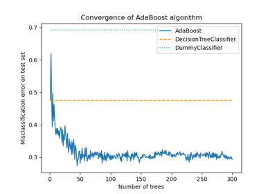
Because the plot shows test-set error repeatedly across model sizes, treat it as an illustration, not as a procedure for choosing your own model. Make development choices using validation data, then reserve your test set for the final check.
Build and compare a majority baseline
Return to the fraud example from last lesson. There are 1,000 illustrative validation transactions: 50 fraudulent and 950 normal. Let 1 mean “flag for review.” Suppose the training labels also have a normal majority. Scikit-learn’s DummyClassifier can learn which label is most frequent from the training labels while ignoring the feature values.
The code below is a worked comparison, not an experiment on a real dataset. Its labels and Policy A predictions are constructed to reproduce last lesson’s counts. In a project, you would replace them with your actual training labels, validation labels, and learned model’s predictions.
from sklearn.dummy import DummyClassifier
from sklearn.metrics import confusion_matrix

# Illustrative training labels: 95 normal, 5 fraud.
y_train = [0] * 95 + [1] * 5

# Placeholder features: the dummy classifier ignores their values.
X_train = [[0]] * len(y_train)

# Constructed validation cases and Policy A predictions from last lesson.
y_val = [1] * 50 + [0] * 950
X_val = [[0]] * len(y_val)
policy_a_pred = [1] * 40 + [0] * 10 + [1] * 95 + [0] * 855

baseline = DummyClassifier(strategy="most_frequent")
baseline.fit(X_train, y_train)
baseline_pred = baseline.predict(X_val)

def results(predictions):
    tn, fp, fn, tp = confusion_matrix(
        y_val, predictions, labels=[0, 1]
    ).ravel()
    return {
        "accuracy": (tp + tn) / len(y_val),
        "recall": tp / (tp + fn),
        "false_positive_rate": fp / (fp + tn),
        "estimated_cost": 100 * fn + 10 * fp,
    }

print("Majority baseline:", results(baseline_pred))
print("Policy A:", results(policy_a_pred))
The resulting comparison is:
| Validation measure | Majority baseline | Policy A |
|---|---|---|
| Accuracy | 95% | 89.5% |
| Recall | 0% | 80% |
| False positive rate | 0% | 10% |
| Estimated error cost | 5,000 units | 1,950 units |
The baseline leaves all 950 normal transactions alone but misses all 50 frauds. Policy A has lower accuracy, yet under last lesson’s illustrative costs—100 units per missed fraud and 10 per unnecessary flag—it has substantially lower estimated cost. Its 10% false positive rate also tells you what that improvement demands of the review process. The baseline makes the trade-off visible rather than letting accuracy decide it silently.
In real use, fit the baseline only on training data. Evaluate it and the learned model on the same validation examples, with the same target definition and cost assumptions. If a baseline uses a rule with a chosen cutoff, establish that cutoff using training or validation data—not the final test set. If cases are ordered in time, preserve the time-aware split you designed earlier rather than randomly mixing future cases into training.
Match the baseline to the task
The majority-class rule fits classification, but other outputs call for other simple predictions. In regression—predicting a number such as a price—a constant prediction can be the training set’s mean or median. You then compare its errors with a model that uses input features. For mean absolute error, a median prediction is often a sensible constant benchmark, particularly when extreme values pull the mean away from a typical case.
Read the relevant portion of the scikit-learn MOOC’s Comparing model performance with a simple baseline. Its housing example shows a DummyRegressor predicting a training-set mean and a decision tree obtaining a lower mean absolute error. The notebook uses repeated validation splits; its “testing errors” within that procedure are not a reason to tune against your reserved final test set.
Comparing model performance with a simple baseline
Read Comparing model performance with a simple baseline from the scikit-learn MOOC to see the same comparison principle applied to numerical predictions.
Start with the introductory paragraph under the page title, from the setup. Then, in the code-and-results portion, find “Then, we evaluate our baseline.” Read the comparison, scanning past the long table of split-by-split values to its interpretation. Finally read the median note. Stop before “Finally, let us see what happens if we measure the test score using” the other metric.
Whether the output is a class or a number, the same standard applies: a meaningful baseline is simple enough to understand, but relevant enough to challenge the proposed model. Beating a dummy predictor shows that features may help. Beating an existing rule is stronger evidence that the new approach improves the current decision. Neither result, by itself, proves the improvement is worth added complexity, operating cost, or risk.
Key takeaways
Build a baseline by specifying a simple prediction rule, deriving anything it needs from training data only, and evaluating it on the same validation cases and decision-relevant measures as your proposed model. Start with a feature-ignoring predictor, then include a current rule or process when one exists. A model should improve the outcome that matters—not merely report a more impressive-looking score.
You have now completed the applied foundations module. Next, you’ll turn a raw product question into an explicit dataset of features and targets, where these baselines can serve as the first checks on whether learning from the data adds value.