Resonance and Breit-Wigner in Scattering

Recommended resources

The freely available resources this lesson will direct you to.

Hello! Let's dive into the next fascinating topic in our study of scattering theory.

In our last lesson, we developed the powerful method of partial wave analysis, seeing how the entire effect of a scattering potential is encoded in a set of phase shifts, ${δ_{l}}$ . We even had a sneak peek at today's topic in a mini-exercise, where we discovered that the scattering cross-section for a given partial wave, $σ_{l}$ , is maximized when the phase shift $δ_{l}$ is an odd multiple of $π /2$ . This special condition is the hallmark of a resonance.

This lesson is dedicated to analyzing these resonance phenomena and deriving the famous Breit-Wigner formula that describes them. We'll explore the deep physical meaning behind resonances: they are signatures of temporary, unstable "quasi-bound" states. This concept is not just a theoretical curiosity; it's fundamental to understanding everything from neutron scattering in nuclear reactors to the discovery of new elementary particles like the Higgs boson at the LHC.

1. The Physical Picture of a Resonance

What exactly is a resonance? Imagine a potential that has a "well" region but doesn't support true bound states for positive energy. This could be a potential well protected by a barrier, as shown in the figure below.

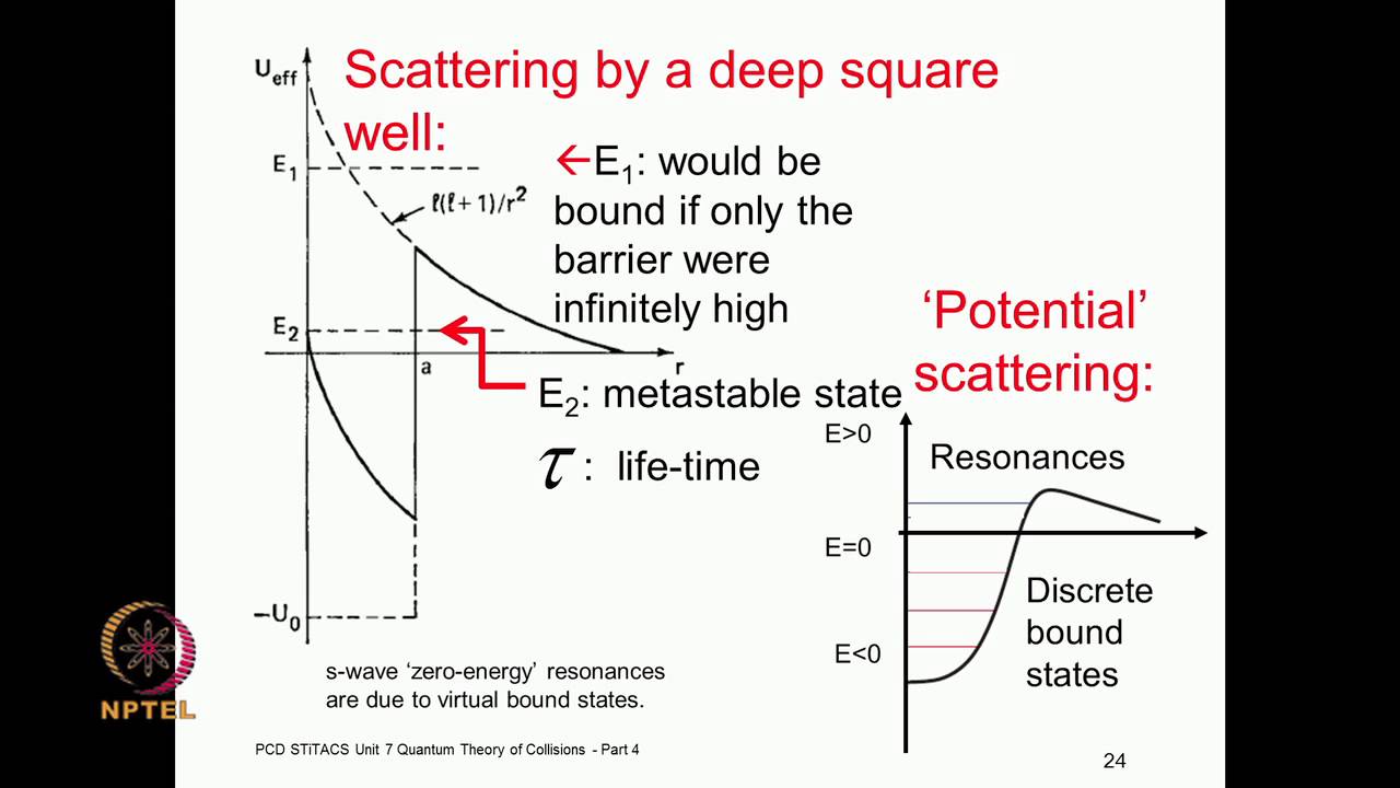
Scattering by a Deep Square Well and Potential Scattering Resonances — On the left, an effective potential with a barrier. A particle with energy $E_2 > 0$ cannot be truly bound. However, it can be temporarily trapped inside the well, forming a metastable state with a finite lifetime $\tau$. On the right, this appears as a sharp peak, or resonance, in the scattering cross-section at energy $E_2$.

If an incoming particle has an energy that happens to match a quasi-stable energy level inside this well, it can get "stuck" there for a relatively long time before eventually escaping (e.g., by tunneling through the barrier). This temporary capture and subsequent release leads to a sharp peak in the scattering cross-section at that specific energy.

This "lingering" of the particle in the potential region has a direct effect on the phase of the scattered wave. A long time delay, $Δ t$ , is related to a rapid change of the phase shift $δ$ with energy $E$ :

Δ t = 2ℏ \frac{d δ}{d E}

Near a resonance, the phase shift changes very rapidly, passing through $π /2$ , which leads to a large time delay and a spike in the cross-section. The constructive interference of waves multiply scattering within the potential, as we will see, is the underlying wave mechanism.

To get a more visceral feel for this, let's watch a segment of a lecture that explains resonance by summing up the amplitudes for multiple scattering paths.

Lecture 14: Resonance and the S-Matrix

In this video, the lecturer from MIT OpenCourseWare provides a fantastic quantum mechanical explanation for resonance. He shows that perfect transmission (a key feature of resonance in 1D) arises from the constructive interference of many different scattering pathways: transmitting directly, transmitting after two reflections, after four reflections, and so on.

Please watch from 16:19 to 22:14. The key takeaway is that resonance isn't just a particle getting 'stuck'; it's a wave phenomenon where multiple scattering amplitudes add up in phase, leading to a dramatic effect.

2. Resonances as Poles of the S-Matrix

While phase shifts are intuitive, a more powerful and general way to think about scattering is through the S-matrix, which relates incoming states to outgoing states. For a single partial wave $l$ , the S-matrix element is simply $S_{l} (k) = e^{2 i δ_{l} (k)}$ .

A profound insight in quantum mechanics is that the stable and metastable states of a system are encoded as poles of the S-matrix when its argument (energy or momentum) is analytically continued into the complex plane.

Poles and Bound States

First, let's see how true, stable bound states appear. A bound state corresponds to a pole of the S-matrix on the positive imaginary axis of the complex momentum plane, i.e., at $k = iκ$ where $κ > 0$ . Why? A state with momentum $k = iκ$ has a spatial dependence $e^{ik x} = e^{- κ x}$ , which is an exponentially decaying, normalizable wavefunction—the defining characteristic of a bound state. Its energy is negative: $E = \frac{ℏ ^{2} k ^{2}}{2 m} = - \frac{ℏ ^{2} κ ^{2}}{2 m}$ .

The following video segment provides an elegant demonstration of this connection.

Lecture 14: Resonance and the S-Matrix

Continuing with the MIT lecture, this part shows how the requirement for a normalizable bound state (with E < 0) forces the incoming amplitudes to be zero, which can only be satisfied if the S-matrix has a pole at that specific energy. This connects the scattering data (S-matrix) to the internal structure of the potential (its bound states).

Please watch from 1:16:27 to 1:23:53. Focus on the main argument: a bound state requires decaying wavefunctions at infinity. This condition, when applied to the S-matrix formalism, implies a divergence (a pole) in the S-matrix elements at the bound state energy.

Poles and Resonances

So, if poles on the imaginary k-axis are bound states, what are resonances? Resonances correspond to poles in the lower half of the complex energy plane (or the corresponding quadrant in the momentum plane).

To understand what this means, let's study a clear and concise explanation from Prof. David Tong's lecture notes.

10. Scattering Theory

These notes on scattering theory from the University of Cambridge explain how poles of the S-matrix give rise to resonances. This section is key to understanding the theoretical underpinnings of our lesson.

Please read the section '10.1.5 Resonances' (pages 313-314). Pay close attention to how a complex energy, E = E_0 - i\Gamma/2, leads to a wavefunction that decays exponentially in time (\propto e^{-\Gamma t/2\hbar}). This is the signature of an unstable, decaying state.

As the reading explains, a pole at a complex energy $E = E_{0} - i Γ/2$ has a profound physical interpretation:

The real part, $E_{0}$ , is the resonant energy—the energy at which the cross-section will peak.
The imaginary part, $- Γ/2$ , dictates the temporal decay. The probability density of the state, $∣ ψ ∣^{2}$ , decays as $e^{- Γ t /ℏ}$ . This means $Γ$ is the width of the resonance, and it is inversely related to the lifetime of the metastable state: $τ = \frac{ℏ}{Γ}$

This is a beautiful manifestation of the energy-time uncertainty principle! A state that exists for a finite time $τ$ cannot have a perfectly defined energy; its energy has an inherent uncertainty or width $Γ$ .

3. The Breit-Wigner Formula

We now have all the pieces to derive the formula that describes the shape of a resonance peak. We know that at a resonance energy $E_{0}$ , the phase shift $δ_{l}$ for the corresponding partial wave passes through $π /2$ . Let's see what this implies for the cross-section.

The contribution of the $l$ -th partial wave to the total cross-section is:

σ_{l} (E) = \frac{4 π}{k ^{2}} (2 l + 1) sin^{2} δ_{l} = \frac{4 π}{k ^{2}} (2 l + 1) \frac{1}{1 + cot ^{2} δ _{l}}

Near the resonance energy $E_{0}$ , we can Taylor-expand $cot δ_{l} (E)$ around $E_{0}$ . Since $δ_{l} (E_{0}) = π /2$ , we have $cot δ_{l} (E_{0}) = 0$ . The first-order expansion is:

cot δ_{l} (E) \approx (E - E_{0}) [\frac{d}{d E} (cot δ_{l})]_{E = E_{0}}

Using the chain rule, $\frac{d}{d E} (cot δ_{l}) = - \frac{1}{s i n ^{2} δ _{l}} \frac{d δ _{l}}{d E}$ . At $E = E_{0}$ , $sin^{2} δ_{l} = 1$ , so we get:

cot δ_{l} (E) \approx - (E - E_{0}) [\frac{d δ _{l}}{d E}]_{E = E_{0}}

We now define the width $Γ$ in terms of this derivative, consistent with our time-delay intuition:

[\frac{d δ _{l}}{d E}]_{E = E_{0}} \equiv \frac{2}{Γ}

Substituting this in gives the simple approximation for $cot δ_{l}$ near resonance:

cot δ_{l} (E) \approx - \frac{2}{Γ} (E - E_{0})

Plugging this back into our formula for $σ_{l}$ , we arrive at the celebrated Breit-Wigner formula:

σ_{l} (E) \approx \frac{4 π}{k ^{2}} (2 l + 1) \frac{( Γ/2 ) ^{2}}{( E - E _{0} ) ^{2} + ( Γ/2 ) ^{2}}

This formula describes a Lorentzian peak centered at $E_{0}$ with a full width at half maximum (FWHM) of exactly $Γ$ . It beautifully quantifies the shape of resonance peaks observed in experiments.

Energy Dependence of Unitary Breit-Wigner Scattering Amplitudes — An example of resonance peaks described by the Breit-Wigner formula for different scattering channels. The characteristic Lorentzian shape is clearly visible.

Test your understanding!

The Z boson, one of the carriers of the weak force, was discovered as a resonance in electron-positron scattering. Its resonance peak is centered at $E_{0} \approx 91.2$ GeV and has a measured width of $Γ \approx 2.5$ GeV. Using the relationship $τ = ℏ/Γ$ , calculate the approximate lifetime of the Z boson in seconds. (You'll need $ℏ \approx 6.582 \times 1 0^{- 16}$ eV·s).

Show answer

First, convert the width from GeV to eV: $Γ = 2.5 GeV = 2.5 \times 1 0^{9} eV$ .
Now, apply the formula:

τ = \frac{ℏ}{Γ} = \frac{6.582 \times 1 0 ^{- 16} eV\cdots}{2.5 \times 1 0 ^{9} eV} \approx 2.63 \times 1 0^{- 25} s

This incredibly short lifetime is why the Z boson is not found freely in nature and can only be observed as a fleeting resonance in high-energy collisions.

To see how this formula is used in practice and its connection to modern physics, let's return to Prof. Tong's notes.

10. Scattering Theory

This section of the notes applies the Breit-Wigner formula to 3D scattering and provides striking examples from particle physics.

Please read section '10.2.7 Resonances' (pages 333-335). It re-derives the Breit-Wigner cross-section from the S-matrix pole and then shows the actual experimental data for the Z boson and the Higgs boson, which are textbook examples of Breit-Wigner resonances.

Conclusion

In this lesson, we have demystified the concept of resonance in quantum scattering, connecting it to the formation of temporary, metastable states. We've seen how this physical picture is rigorously described in the language of complex analysis, where resonances appear as poles of the S-matrix.

Key Takeaways:

A resonance is a sharp peak in the scattering cross-section that occurs when an incident particle's energy matches that of a quasi-bound state of the potential.
The lifetime of this metastable state, $τ$ , is related to the energy width of the resonance, $Γ$ , by the uncertainty principle: $τ = ℏ/Γ$ .
The shape of the resonance peak is described by the Breit-Wigner formula, which has a characteristic Lorentzian profile.
In the S-matrix formalism, bound states correspond to poles on the positive imaginary momentum axis ( $E < 0$ ), while resonances correspond to poles in the lower half of the complex energy plane ( $E = E_{0} - i Γ/2$ ).

Preview of the Next Lesson:
We've seen that the S-matrix must be unitary ( $S^{†} S = 1$ ), which reflects the conservation of probability. This has deep consequences. In the next lesson, we will derive one of the most important of these: the Optical Theorem. This theorem provides a surprising and powerful link between the total scattering cross-section and the imaginary part of the forward scattering amplitude, $f (θ = 0)$ .