Ising Model Exponents: Exact vs. Mean-Field

Recommended resources

The freely available resources this lesson will direct you to.

Hello! Welcome back to our investigation of the Ising model.

In our last lesson, we reached a major milestone by stating Onsager's exact solution for the free energy of the 2D Ising model. By analyzing this solution, we uncovered its profound physical consequences: a genuine phase transition at a finite temperature $T_{c}$ , marked by a logarithmic divergence in the specific heat ( $α = 0$ ) and a spontaneous magnetization that vanishes as $(T_{c} - T)^{1/8}$ ( $β = 1/8$ ). We noted that these results were distinctly different from the predictions of simpler theories.

Today, we will build directly on that foundation. Our goal is to complete the set of standard critical exponents for the 2D Ising model and then conduct a systematic, quantitative comparison with the exponents derived from mean-field theory. This contrast is a cornerstone of modern statistical physics, as it precisely illuminates why mean-field approximations fail in low dimensions and highlights the crucial role of fluctuations near a critical point.

This lesson directly addresses the learning outcome: Identify the critical exponents from the exact 2D Ising model solution and contrast them with mean-field values.

A Quick Recap: Defining Critical Exponents

As a reminder, critical exponents describe the singular power-law behavior of thermodynamic quantities as the system approaches a critical point. We typically express this in terms of the reduced temperature, $t = (T - T_{c}) / T_{c}$ . If a quantity $Q$ diverges as $t \to 0$ , we write $Q \sim ∣ t ∣^{- E}$ , and if it vanishes, we write $Q \sim ∣ t ∣^{E}$ , where $E$ is the critical exponent.

Part 1: The Full Set of 2D Ising Exponents

In the previous lesson, we found the exponents for the specific heat ( $α$ ) and the spontaneous magnetization ( $β$ ). Now, let's introduce the other key exponents and state their exact values for the 2D Ising model. These values are derived from highly non-trivial analyses of the exact solution and related correlation functions, which are beyond the scope of our course.

To understand these exponents, we can read a concise summary from the text "The Onsager Solution and Exact Series Expansions".

The Onsager Solution and Exact Series Expansions

This section of the textbook chapter provides a clear definition of the common critical exponents and lists their exact values for the 2D Ising model. It's an excellent summary of the results we will be discussing.

Please read the section '5.5 Singularities, Critical Exponents, and Universality'. Focus on the definitions of the exponents α, β, and γ, and note the values given for the 2D case in the text and in Table 5.1.

Based on that reading and other established results, the full set of critical exponents for the 2D Ising model is:

Specific Heat ( $α$ ): Describes the divergence of the specific heat at zero field, $C_{H} \sim ∣ t ∣^{- α}$ .
- 2D Ising Value: $α = 0$ . This notation signifies a logarithmic divergence, $C_{H} \sim - ln ∣ t ∣$ , which is a weaker singularity than any power law.
Order Parameter ( $β$ ): Describes how the spontaneous magnetization vanishes as $T$ approaches $T_{c}$ from below, $M_{0} \sim (- t)^{β}$ for $t < 0$ .
- 2D Ising Value: $β = 1/8$ .
Susceptibility ( $γ$ ): Describes the divergence of the magnetic susceptibility, $χ = (\partial M / \partial H)_{T} \sim ∣ t ∣^{- γ}$ , as $H \to 0$ .
- 2D Ising Value: $γ = 7/4$ .
Critical Isotherm ( $δ$ ): Describes the relationship between magnetization and field exactly at the critical temperature, $H \sim ∣ M ∣^{δ} sgn (M)$ at $t = 0$ .
- 2D Ising Value: $δ = 15$ .
Correlation Length ( $ν$ ): Describes the divergence of the correlation length $ξ$ , which is the characteristic length scale of spin-spin correlations, $ξ \sim ∣ t ∣^{- ν}$ .
- 2D Ising Value: $ν = 1$ .
Correlation Function ( $η$ ): Describes the power-law decay of the correlation function $G (r) = ⟨ s_{0} s_{r} ⟩ - ⟨ s_{0} ⟩ ⟨ s_{r} ⟩$ exactly at $T_{c}$ , where it decays as $G (r) \sim 1/ r^{d - 2 + η}$ .
- 2D Ising Value: $η = 1/4$ .

This set of numbers—(0, 1/8, 7/4, 15, 1, 1/4)—represents a precise, quantitative fingerprint of the critical point in the 2D Ising universality class.

Part 2: Calculating the Mean-Field Exponents

Now, let's derive the corresponding exponents from mean-field theory (MFT). We will explore MFT in depth in the next module, but for now, we can use its central result: the expanded equation of state near $T_{c}$ .

A clear derivation of these exponents is available in the following notes.

[PDF] 1 Unit 4-4: Critical Exponents within the Mean-Field Approximation ...

This document provides a concise, step-by-step analytical derivation of the mean-field critical exponents from the expanded self-consistency equation. It's an ideal resource for our current goal.

Please read through the derivations for each exponent. The key starting point is Equation 4.4.7, which gives the magnetic field h as a function of magnetization m and temperature T near the critical point. Follow how this single equation is used to extract β, δ, γ, and α.

Let's summarize the derivations. The MFT equation of state near the critical point can be written as:

h \approx A t m + B m^{3}

where $h$ is proportional to the magnetic field, $m$ is the magnetization, $t = (T - T_{c}) / T_{c}$ , and $A, B$ are positive constants. This equation contains all the critical behavior in MFT.

Exponent $β$ : For spontaneous magnetization, we set $h = 0$ and consider $t < 0$ .
$0 = A t m + B m^{3} ⟹ m^{2} = - \frac{A}{B} t$
So, $m \sim (- t)^{1/2}$ . This gives $β = 1/2$ .
Exponent $δ$ : At the critical temperature, $t = 0$ .
$h \approx B m^{3}$
This gives $δ = 3$ .
Exponent $γ$ : The susceptibility is $χ = (\partial m / \partial h)_{t}$ . It's easier to compute its inverse: $χ^{- 1} = (\partial h / \partial m)_{t} = A t + 3 B m^{2}$ .
- For $t > 0$ , the equilibrium state is $m = 0$ , so $χ^{- 1} = A t$ . Thus $χ \sim t^{- 1}$ .
- For $t < 0$ , the spontaneous magnetization is $m^{2} = - A t / B$ . Substituting this in, $χ^{- 1} = A t + 3 B (- A t / B) = A t - 3 A t = - 2 A t$ . Thus $χ \sim (- t)^{- 1}$ .
  In both cases, the exponent is 1. This gives $γ = 1$ .
Exponent $α$ : As shown in the resource, calculating the free energy and then the specific heat $c \sim - T (\partial^{2} f / \partial T^{2})$ reveals a finite jump at $T_{c}$ , but no divergence. A finite jump corresponds to $α = 0$ .
Exponents $ν$ and $η$ : These are derived from the spatial correlations, which are absent in the simplest form of MFT. A more advanced treatment (Landau-Ginzburg theory, which we'll see in Module 6) shows that MFT corresponds to $ν = 1/2$ and $η = 0$ . The value $η = 0$ means that correlations at $T_{c}$ decay as $1/ r^{d - 2}$ , the classical Ornstein-Zernike form.

Test your understanding!

The relationship $γ = β (δ - 1)$ is a famous scaling relation. Verify that the mean-field exponents $β = 1/2$ , $γ = 1$ , and $δ = 3$ satisfy this relation.

Show answer

Let's plug the mean-field values into the right-hand side of the equation:
$β (δ - 1) = \frac{1}{2} (3 - 1) = \frac{1}{2} (2) = 1$
This result, 1, is precisely the mean-field value for $γ$ . So, the relation holds. In Module 7, we'll see that these scaling relations are a deep consequence of the physics of critical phenomena and must be satisfied by any valid set of exponents. The 2D Ising exponents ( $γ = 7/4$ , $β = 1/8$ , $δ = 15$ ) also satisfy this relation: $1/8 \times (15 - 1) = 14/8 = 7/4$ .

Part 3: The Contrast

We now have two complete sets of fingerprints for a critical point. Let's place them side-by-side.

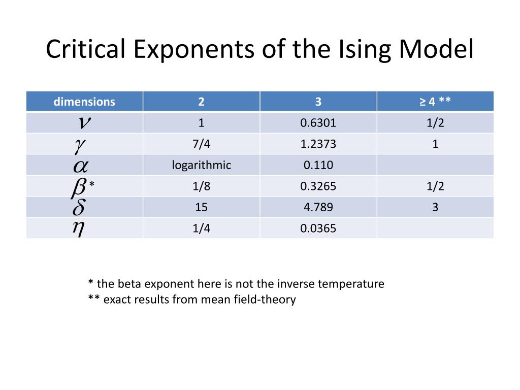
Critical Exponents of the Ising Model — This table summarizes the critical exponents for the Ising model in different dimensions. The 2D values come from the exact solution, while the values for d$\ge$4 are the mean-field exponents we just derived. (The 3D values are from numerical simulations and series expansions).

Let's organize this into our own table for clarity:

Exponent	Physical Quantity	Mean-Field Theory Value	Exact 2D Ising Value
$α$	Specific Heat ( $C_{H}$ )	0 (finite jump)	0 (logarithmic $\infty$ )
$β$	Magnetization ( $M_{0}$ )	1/2	1/8
$γ$	Susceptibility ( $χ$ )	1	7/4
$δ$	Critical Isotherm ( $H \sim M^{δ}$ )	3	15
$ν$	Correlation Length ( $ξ$ )	1/2	1
$η$	Correlation Decay at $T_{c}$	0	1/4

The discrepancy is not subtle; it is dramatic. Every single exponent is different.

Qualitative vs. Quantitative Failure: MFT correctly predicts a singularity exists, but it gets the nature of that singularity completely wrong in two dimensions. The difference between a finite jump ( $α_{MFT} = 0$ ) and a logarithmic divergence ( $α_{2 D} = 0$ ) is profound.
Strength of Divergences: The 2D Ising exponents for susceptibility ( $γ = 7/4 > 1$ ) and correlation length ( $ν = 1 > 1/2$ ) are larger than their MFT counterparts. This indicates that fluctuations and the range of correlations diverge much more violently near the critical point than MFT predicts.
Shape of the Transition: The difference in $β$ is visually striking. A $β = 1/2$ curve is rounded, while a $β = 1/8$ curve is much flatter, dropping to zero more abruptly near $T_{c}$ .

Comparison of Magnetization: Simulation vs. Mean Field Prediction — This graph illustrates the difference in the order parameter's behavior. The blue line shows a typical mean-field curve with a gentle slope near $T_c$ (related to $\beta=1/2$). The red points, representing a simulation that captures fluctuations (and is qualitatively similar to the 2D exact result), show a much steeper approach to zero (related to $\beta=1/8$).

The fundamental reason for this disagreement lies in the core approximation of mean-field theory: it replaces the interactions of a given spin with its fluctuating neighbors with an interaction with a single, non-fluctuating average or mean field. This approximation completely neglects the correlated fluctuations that become dominant near a critical point, where the correlation length $ξ$ diverges. The exact solution for the 2D Ising model fully incorporates these fluctuations, leading to the correct, non-trivial exponents.

Conclusion

In this lesson, we have completed our survey of the critical exponents for the 2D Ising model and contrasted them with the predictions of mean-field theory.

Key Takeaways:

There is a standard set of critical exponents ( $α, β, γ, δ, ν, η$ ) that characterize the nature of a continuous phase transition.
The exact values for the 2D Ising model are $α = 0$ (log), $β = 1/8$ , $γ = 7/4$ , $δ = 15$ , $ν = 1$ , and $η = 1/4$ .
Mean-field theory predicts a different, "classical" set of exponents: $α = 0$ (jump), $β = 1/2$ , $γ = 1$ , $δ = 3$ , $ν = 1/2$ , and $η = 0$ .
The stark difference between these two sets reveals the quantitative failure of mean-field theory in low dimensions ( $d = 2$ ) and underscores the essential role of long-range fluctuations in determining critical behavior.

Preview of the Next Module:
We have now concluded our module on the Ising model and its exact solutions. We have repeatedly used mean-field theory as a point of comparison. In the next module, we will put mean-field theory itself under the microscope. We will begin by formally deriving the mean-field equation for the Ising model using the "molecular field" approximation, providing a solid foundation for the results we have used today and a deeper understanding of the theory's strengths and limitations.