Onsager's Solution for 2D Ising Model Free Energy

Recommended resources

The freely available resources this lesson will direct you to.

Hello! Welcome back to our study of the Ising model.

In the last lesson, we took a significant step by extending the transfer matrix method to the two-dimensional Ising model. We saw how the problem of calculating the partition function for a 2D classical system could be mapped onto finding the largest eigenvalue of a $2^{N} \times 2^{N}$ transfer matrix, which itself is equivalent to studying the ground state of a 1D quantum spin chain. This established the machinery for a full solution. Finding the eigenvalues of that enormous matrix, however, remained an unsolved challenge.

Today, we will jump to the historic resolution of this challenge. We will state and analyze the celebrated exact solution for the free energy of the 2D Ising model, first derived by Lars Onsager in 1944. This was a monumental achievement in theoretical physics, providing the first exact description of a system with a continuous phase transition and non-trivial critical behavior. Our goal is to understand the form of this solution and its profound physical implications.

This lesson directly addresses the learning outcome: to state Onsager's exact solution for the free energy of the 2D Ising model. We will not reproduce the famously complex derivation, but we will examine the result in detail to uncover the physics it contains.

A Note on the Derivation

Before we present the solution, it's worth appreciating the difficulty of its discovery. Onsager's original 1944 paper used the transfer matrix formalism we developed, but solving for the eigenvalues required sophisticated algebraic techniques involving Lie algebras, which were not widely known among physicists at the time. Since then, other, more transparent (though still highly advanced) methods have been developed.

The following video provides an excellent high-level overview of the problem and the significance of Onsager's achievement. It also briefly touches upon the complexity of the derivation methods.

The hardest sum aka the Ising model #SoME3

Watch this segment from the Number Cruncher channel to get a sense of the scale of the problem and the elegance of the final solution. It also mentions the different approaches used to solve it.

Please watch from 28:39 to 33:33. The first part (28:39 - 31:25) visually shows how the behavior of thermodynamic quantities like specific heat sharpens as the system size increases, culminating in the singular behavior of the infinite lattice solution. The second part (31:25 - 33:33) discusses the immense mathematical challenge of the derivation itself.

As the video illustrates, the solution is surprisingly compact, even if the path to it is not. Let's now look at that final result.

The Exact Solution for the Free Energy

Onsager's solution gives the free energy per site, $f = F / N$ , in the thermodynamic limit ( $N \to \infty$ ) for the 2D Ising model on a square lattice with zero external magnetic field ( $H = 0$ ). The result is expressed as an integral over the Brillouin zone of the reciprocal lattice.

A clear presentation of this result can be found in the lecture notes from the "Universality in condensed matter" course.

Ising model and phase transitions

These notes directly present Onsager's solution for the free energy on square, triangular, and hexagonal lattices. We will focus on the square lattice case.

Please read the section '5.3.2 2d Ising model onsager’s solution', focusing on Equation 5.40 and the subsequent analysis for the square lattice. Pay attention to how the critical temperature is found from the condition that the argument of the logarithm becomes zero.

As stated in the resource, the free energy per spin for the square lattice is:

f (T, 0) = - k_{B} T ln 2 - \frac{k _{B} T}{2} \int_{- π}^{π} \frac{d ^{2} k}{( 2 π ) ^{2}} ln [cosh^{2} (2 K) - sinh (2 K) (cos k_{x} + cos k_{y})]

where $K = J / k_{B} T$ as usual, and we have set the lattice spacing to unity.

This equation is the heart of today's lesson. It contains all the thermodynamic information about the zero-field 2D Ising model. Our task is to extract the physics.

Locating the Phase Transition

A phase transition manifests as a non-analyticity in the free energy. In the expression above, the only possible source of a non-analyticity is the logarithm. The integral will be non-analytic if the argument of the logarithm becomes zero or negative for any value of $(k_{x}, k_{y})$ in the domain of integration.

The argument of the logarithm is:

P (T, k) = cosh^{2} (2 K) - sinh (2 K) (cos k_{x} + cos k_{y})

We need to find the condition under which $P (T, k)$ is minimized. Since $sinh (2 K) > 0$ for $T > 0$ , the term $- sinh (2 K) (cos k_{x} + cos k_{y})$ is minimized when $(cos k_{x} + cos k_{y})$ is maximized. The maximum value is 2, which occurs at $k = (0, 0)$ .

Therefore, a singularity will first appear when the argument of the log becomes zero at $k = (0, 0)$ . The critical temperature, $T_{c}$ , is determined by the condition $P (T_{c}, 0) = 0$ :

cosh^{2} (2 K_{c}) - sinh (2 K_{c}) (1 + 1) = 0

where $K_{c} = J / k_{B} T_{c}$ . This simplifies to:

cosh^{2} (2 K_{c}) = 2 sinh (2 K_{c})

Using $cosh^{2} (x) = 1 + sinh^{2} (x)$ , we get a quadratic equation for $sinh (2 K_{c})$ :

sinh^{2} (2 K_{c}) - 2 sinh (2 K_{c}) + 1 = 0 ⟹ (sinh (2 K_{c}) - 1)^{2} = 0

This gives the famous condition for the critical point of the 2D Ising model:

sinh (\frac{2 J}{k _{B} T _{c}}) = 1

Solving for $T_{c}$ yields:

\frac{k _{B} T _{c}}{J} = \frac{2}{arsinh ( 1 )} = \frac{2}{ln ( 1 + 2 )} \approx 2.269

This is a precise, non-trivial prediction, a landmark result that confirmed the existence of a finite-temperature phase transition and provided its exact location.

Consequences of the Solution: Thermodynamic Quantities

With the exact free energy, we can calculate its derivatives to find other thermodynamic quantities and see how they behave at $T_{c}$ .

Specific Heat

The specific heat at constant volume (and zero field) is given by $C = - T (\partial^{2} F / \partial T^{2})$ . While the full calculation is involved, the analysis of the integral near $T_{c}$ shows that the specific heat diverges logarithmically:

C (T) \sim - \frac{8 k _{B}}{π} (\frac{J}{k _{B} T _{c}})^{2} ln ∣ t ∣ as t \to 0

where $t = (T - T_{c}) / T_{c}$ is the reduced temperature. This logarithmic divergence is a hallmark of the 2D Ising model.

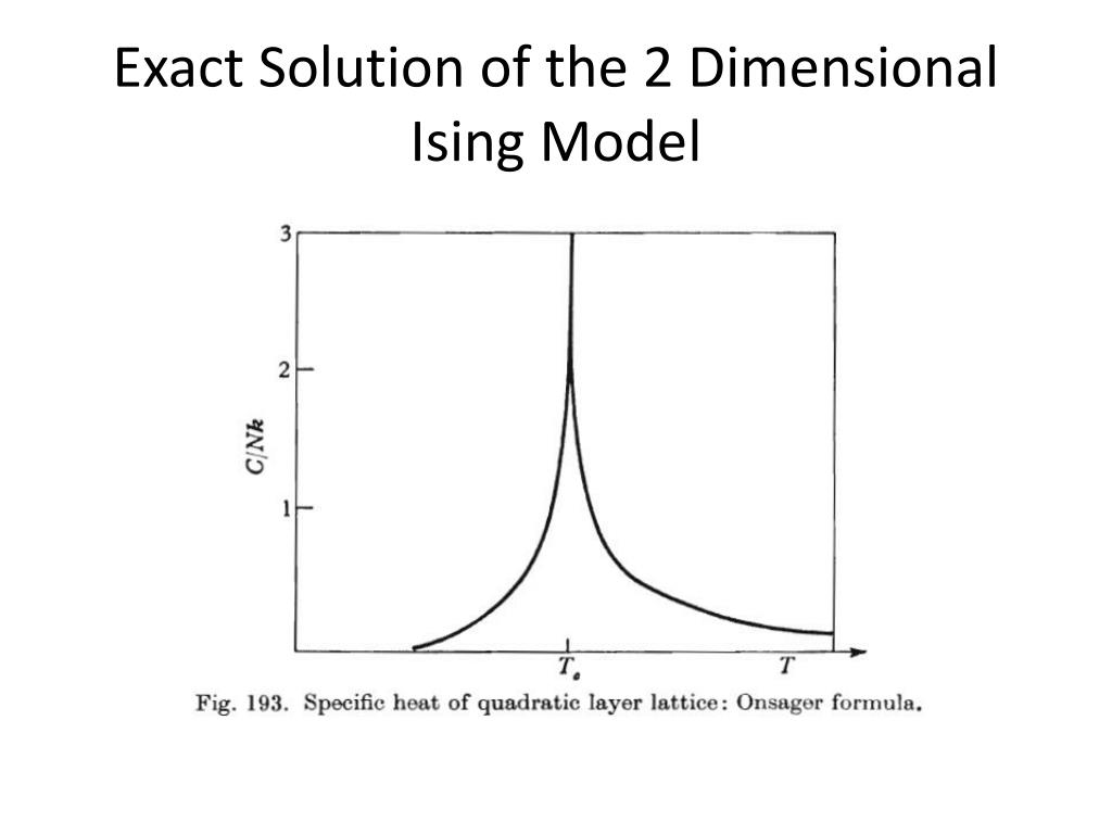
Specific Heat from Onsager's Exact Solution for the 2D Ising Model — This graph shows the specific heat per particle for the 2D Ising model on a square lattice, as derived from Onsager's solution. The sharp, symmetric logarithmic divergence at the critical temperature $T_c$ is clearly visible. This behavior is fundamentally different from the simple finite jump predicted by mean-field theory.

This logarithmic divergence means the critical exponent $α$ , defined by $C \sim ∣ t ∣^{- α}$ , is $α = 0$ . (A power-law divergence corresponds to $α > 0$ , while a simple cusp corresponds to $α < 0$ ).

Test your understanding!

In the previous module, we found that the mean-field critical exponents for the Van der Waals gas were $α = 0$ (for specific heat at constant volume), $β = 1/2$ , $γ = 1$ , and $δ = 3$ . The 2D Ising model also has $α = 0$ . Does this mean the specific heat behaves the same way in both models near $T_{c}$ ?

Show answer

No, the behavior is different. In mean-field theory (like the Van der Waals model or the Weiss theory of ferromagnetism), $α = 0$ corresponds to a finite jump or discontinuity in the specific heat at $T_{c}$ . In the 2D Ising model, $α = 0$ signifies a logarithmic divergence at $T_{c}$ . Both fall under the classification $α = 0$ , but the singular behavior is much stronger in the 2D Ising case, indicating the crucial role of fluctuations not captured by mean-field theory.

Spontaneous Magnetization

Onsager's solution is for $H = 0$ . Since the magnetization $M = - (\partial F / \partial H)$ is an odd function of $H$ , it is strictly zero at $H = 0$ for all $T$ . To find the spontaneous magnetization $M_{0}$ , one must calculate the free energy in an infinitesimal positive field $H \to 0^{+}$ for $T < T_{c}$ . This feat was accomplished by C. N. Yang in 1952. The result is:

M_{0} (T) = [1 - sinh^{- 4} (\frac{2 J}{k _{B} T})]^{1/8} for T < T_{c}

Near the critical point, as $T \to T_{c}^{-}$ , this expression simplifies to:

M_{0} (T) \sim (- t)^{1/8}

This gives the critical exponent for the order parameter: $β = 1/8$ . This value is drastically different from the mean-field prediction of $β = 1/2$ , again highlighting the failure of mean-field theory to capture the correct physics in two dimensions.

Conclusion

In this lesson, we have stated and examined one of the cornerstones of statistical physics: Onsager's exact solution for the 2D Ising model.

Key Takeaways:

The exact free energy per site for the 2D Ising model at $H = 0$ is given by a definite integral over the Brillouin zone.
The phase transition occurs as a non-analyticity in the free energy, which arises when the argument of the logarithm in the integrand goes to zero.
This condition precisely determines the critical temperature, giving $sinh (2 J / k_{B} T_{c}) = 1$ .
The specific heat exhibits a logarithmic divergence at $T_{c}$ , corresponding to a critical exponent $α = 0$ .
The spontaneous magnetization vanishes as $(T_{c} - T)^{1/8}$ as the critical temperature is approached from below, giving a critical exponent $β = 1/8$ .

These results provided the first exact, non-mean-field critical exponents and were a crucial step towards the modern theory of critical phenomena, universality, and the renormalization group.

Preview of the Next Lesson:
We have now seen two critical exponents, $α = 0$ and $β = 1/8$ , that differ from their mean-field counterparts. In the next lesson, we will complete this picture by identifying the full set of critical exponents ( $γ, δ, ν, η$ ) from the exact 2D Ising model solution and systematically contrasting them with the universal predictions of mean-field theory. This comparison will underscore the importance of dimensionality and fluctuations in the theory of phase transitions.