Estimating Temperature Trends with Autocorrelation and ENSO

Hello. Last lesson asked whether a temperature record measures climate consistently over time. Now assume you have a global monthly temperature-anomaly series ready to analyse. A rising fitted line is easy to draw; the harder question is how precisely its slope is estimated when neighbouring months share weather patterns and ocean conditions.

In this lesson, you will estimate a warming trend, test it without treating correlated months as independent observations, and examine how an ENSO indicator changes the estimate. The distinction between a measured trend and an explanation for that trend will remain important throughout. Allow roughly 45–50 minutes, including the videos, reading, and Python demonstration.

What a straight-line trend estimates

Let $T_t$ be the global mean temperature anomaly in month $t$. An anomaly is a departure from a specified reference-period average; changing that reference period generally shifts the series vertically without changing its trend. For a chosen interval, fit

where $x_t$ is elapsed time in decades. Then $\beta$ is the fitted change in degrees Celsius per decade. The intercept is mainly bookkeeping: it depends on the reference period and where you set time zero.

Ordinary least squares (OLS) estimates $\beta$ by minimising squared residuals. Testing $H_0:\beta =0$ asks whether the series is compatible, under the statistical model, with no linear trend over this particular interval. It does not ask whether every month warmed, whether the trend was constant outside the interval, or what caused it.

The figure below shows why those qualifications matter. The upper series rises overall but fluctuates substantially. The lower series tracks sea-surface temperature anomalies in the tropical Pacific Niño3.4 region; red and blue mark warm and cool ENSO phases. Compare broad movements rather than expecting corresponding peaks to fall in precisely the same month.

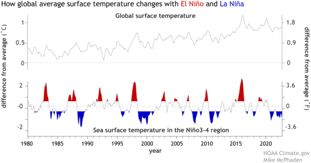
This is an illustration, not a numerical dataset from which to report a defensible slope or $p$-value. An estimate requires the underlying monthly observations, a declared start and end date, and a stated method.

Two different roles for ENSO and serial correlation

ENSO is a coupled ocean–atmosphere pattern in the tropical Pacific. During El Niño, warmer-than-usual water extends across more of the central and eastern Pacific; La Niña strengthens the cooler conditions there. Because these changes cover a large area and affect atmospheric circulation, they can influence global monthly temperature. They are useful for understanding why some months sit above or below a fitted trend.

Serial correlation is a different statistical issue. Even after fitting a trend, a warm residual this month makes a warm residual next month more likely. A simple representation is

where the innovations ${\epsilon }_t$ are uncorrelated and $\rho$ describes persistence. This AR(1) model is a starting point, not an assumption that climate residuals must obey exactly. ENSO can account for some serially patterned variation, while ocean heat storage, other climate processes, or an inadequate trend specification can leave further dependence.

Why does persistence change inference? Adjacent warm months contain less independent information about a decades-long slope than the same number of unrelated measurements would. Under the usual conditions for OLS, serial correlation does not by itself make the fitted slope biased, but the standard OLS standard error and $t$-test rely on an incorrect independence assumption. With positive persistence, treating months as independent commonly makes the slope appear more precisely known than it is. A residual autocorrelation function (ACF) helps diagnose this problem after fitting the proposed trend model.

A trend test with an ENSO covariate and robust uncertainty

Extend the regression by using a Niño3.4 temperature anomaly $E_t$:

Here $E_{t-3}$ is the ENSO index three months earlier. Three months is an illustrative, preselected lag, not a universal physical constant. A positive $\gamma$ would mean that, within this model, warmer Niño3.4 conditions tend to be associated with a warmer subsequent global anomaly.

The two regressions answer related but different descriptive questions:

• Trend only: $\beta$ is the fitted change in the observed global series, including whatever ENSO variation happened during the chosen interval.
• Trend plus ENSO: $\beta$ is the fitted change conditional on the specified ENSO indicator. If ENSO phases are unevenly distributed near the interval’s endpoints, this slope may differ from the trend-only slope.

Neither slope coefficient is, merely by being a regression coefficient, an estimate of the human-caused contribution. ENSO is also measured within the climate system, not assigned independently like a randomised treatment. A conditional trend can help separate short-term variation without establishing physical attribution.

To make the trend test more credible, we can retain the OLS slope but calculate a heteroskedasticity-and-autocorrelation-consistent (HAC) standard error. Unlike the conventional OLS calculation, HAC allows residuals separated by nearby months to be correlated. It requires a choice of how many lags to include; 12 and 24 months are useful sensitivity checks here, not guarantees that all longer dependence has been captured. The resulting confidence intervals and $p$-values are approximate, especially for short samples.

There is a second, subtler limitation. Regressing temperature on time, ENSO, solar activity, and volcanic indicators is sometimes described as “removing natural variability.” Whether that works depends on how the indicators represent the timing and duration of temperature responses, and on whether a straight line adequately represents what remains.

The practical response is not to abandon regression. It is to state what was controlled for, check residual behaviour, and test whether reasonable analysis choices materially change the result.

Implementing the comparison in Python

The code below accepts a CSV named monthly_gmst_enso.csv with columns date, gmst_anomaly_c, and nino34_anomaly_c. Dates should identify consecutive months, and the two series must be aligned. If that file is absent, the code creates a synthetic demonstration with a known rising component, an ENSO-like indicator, and persistent noise. Synthetic output verifies the procedure; it is not an estimate of historical warming.

The three-month lag discards the first three months in both regressions, so changes between their slopes cannot be attributed to comparing different date ranges.

from pathlib import Path

import numpy as np
import pandas as pd
import statsmodels.api as sm
from statsmodels.stats.diagnostic import acorr_ljungbox
from statsmodels.tsa.stattools import acf

path = Path("monthly_gmst_enso.csv")

if path.exists():
    df = pd.read_csv(path, parse_dates=["date"])
    df = df[["date", "gmst_anomaly_c", "nino34_anomaly_c"]]
    print("Using supplied monthly observations")
else:
    rng = np.random.default_rng(14)
    n = 480
    enso = np.zeros(n)
    noise = np.zeros(n)

    for t in range(1, n):
        enso[t] = 0.90 * enso[t - 1] + rng.normal(0, 0.40)
        noise[t] = 0.55 * noise[t - 1] + rng.normal(0, 0.06)

    enso_lag3 = np.r_[np.zeros(3), enso[:-3]]
    temperature = (
        0.18 * np.arange(n) / 120  # 0.18 °C per decade by construction
        + 0.11 * enso_lag3
        + noise
    )
    df = pd.DataFrame({
        "date": pd.date_range("1980-01-01", periods=n, freq="MS"),
        "gmst_anomaly_c": temperature,
        "nino34_anomaly_c": enso,
    })
    print("Using SYNTHETIC data; results are not historical estimates")

df = df.sort_values("date").reset_index(drop=True)
assert df[["gmst_anomaly_c", "nino34_anomaly_c"]].notna().all().all()

month_number = (df["date"].dt.year * 12 + df["date"].dt.month).to_numpy()
assert np.all(np.diff(month_number) == 1), "Supply consecutive months"

df["decades"] = (month_number - month_number[0]) / 120
df["enso_lag3"] = df["nino34_anomaly_c"].shift(3)
d = df.dropna().copy()

y = d["gmst_anomaly_c"]
trend_only = sm.OLS(y, sm.add_constant(d[["decades"]])).fit()
with_enso = sm.OLS(
    y, sm.add_constant(d[["decades", "enso_lag3"]])
).fit()

def report(fit, label):
    slope_index = fit.model.exog_names.index("decades")
    print(f"\n{label}: slope in °C per decade")
    for lag in (0, 12, 24):
        result = (
            fit if lag == 0 else
            fit.get_robustcov_results(cov_type="HAC", maxlags=lag)
        )
        method = "ordinary OLS SE" if lag == 0 else f"HAC, {lag} lags"
        interval = result.conf_int()[slope_index]
        print(
            f"{method:16s} slope={result.params[slope_index]:.3f}"
            f"  SE={result.bse[slope_index]:.3f}"
            f"  95% CI=({interval[0]:.3f}, {interval[1]:.3f})"
            f"  p={result.pvalues[slope_index]:.3g}"
        )

    residual_acf = acf(fit.resid, nlags=24, fft=True)
    print("Residual ACF at lags 1, 12, 24:",
          np.round(residual_acf[[1, 12, 24]], 3))
    print("Ljung–Box p-values for residual correlation through lags 12, 24:")
    print(acorr_ljungbox(
        fit.resid, lags=[12, 24], return_df=True
    )["lb_pvalue"])

report(trend_only, "Trend only")
report(with_enso, "Trend plus ENSO")

enso_hac = with_enso.get_robustcov_results(
    cov_type="HAC", maxlags=24
)
enso_index = with_enso.model.exog_names.index("enso_lag3")
print("\nENSO coefficient and HAC(24) p-value:",
      enso_hac.params[enso_index],
      enso_hac.pvalues[enso_index])

Read the output in this order. First compare the slopes: adding ENSO changes the fitted specification, so it can change the point estimate. Next, within either specification, compare the ordinary and HAC standard errors and intervals: HAC changes the uncertainty calculation, not that model’s OLS slope. Finally inspect the residual ACF and Ljung–Box results. The Ljung–Box null is no residual autocorrelation through the tested lags; rejection warns that dependence remains. Failure to reject does not prove that all dependence is gone.

If you use observations, the CSV must be a global mean temperature-anomaly series rather than values read off the figure. Record the dataset, its date range, its reference period, and any missing-month decisions alongside the result. Try a predeclared alternative ENSO lag and a longer HAC lag range as sensitivity analyses. Selecting whichever lag or interval delivers the smallest $p$-value and reporting only that result would make the stated uncertainty misleading.

What the test can—and cannot—settle

A statistically detectable positive slope says that the data, under the stated trend model and uncertainty method, are inconsistent with a zero linear slope over the selected period. Its numerical size and uncertainty deserve more attention than a significance label alone.

Three checks keep that conclusion proportionate. Shortening or moving the interval can alter the estimate because ENSO episodes and other influences are not evenly distributed across endpoints. Including an ENSO index can reduce one source of fluctuation, but an imperfect lag or an omitted persistent process may remain in the residuals. And a straight line is a summary of a selected interval, not a physical law requiring the climate response to be exactly linear.

These are specification questions as well as standard-error questions. HAC protects against certain errors in estimated precision; it cannot repair a misleading mean model or turn a conditional association into causal attribution.

Conclusion

You can estimate a global temperature trend by fitting anomaly against time measured in decades, then report its slope with a confidence interval. Before trusting a conventional trend test, inspect residual autocorrelation and use an uncertainty method—such as HAC—that accommodates dependence. An ENSO covariate can clarify how short-term Pacific variability affects the fitted result, provided its lag and interpretation are stated openly.

The next lesson applies similar attention to measurement and uncertainty to global mean sea level, where satellite altimetry and tide gauges provide different views of the same changing quantity.