Measuring Global Sea-Level Rise: Methods, Data, and Uncertainty

Hello. Last lesson separated a fitted temperature trend from the uncertainty attached to it. Sea level poses a related statistical problem, but first it poses a measurement problem: a coastal instrument measures water relative to nearby land, while a satellite measures the ocean surface in a reference frame tied to Earth’s centre.

In roughly 40–45 minutes, you will trace how each observation becomes a global mean sea-level record, identify the adjustments that matter, and assess what a reported rise and acceleration can—and cannot—tell you. The distinction between what was measured and what was inferred from it will be useful throughout.

One ocean, two reference frames

Consider the sea surface at a coast. Let $H_t$ denote its height in a reference frame tied to Earth’s centre, and $L_t$ the height of a benchmark on the adjacent land. A tide gauge measures their difference:

Thus a change in relative sea level can reflect water rising, land sinking, or both. If the sea surface rises at $3$ mm/year while the land sinks at $2$ mm/year, the gauge records a relative rise of $5$ mm/year. That is a valid measurement of the changing water level experienced at that coast; it is not, by itself, a measurement of global ocean rise.

A satellite altimeter instead estimates sea-surface height relative to a geocentric reference frame. The observational setup below makes the distinction visible. The coastal benchmark anchors the tide gauge, while positioning satellites help measure movement of the land itself.

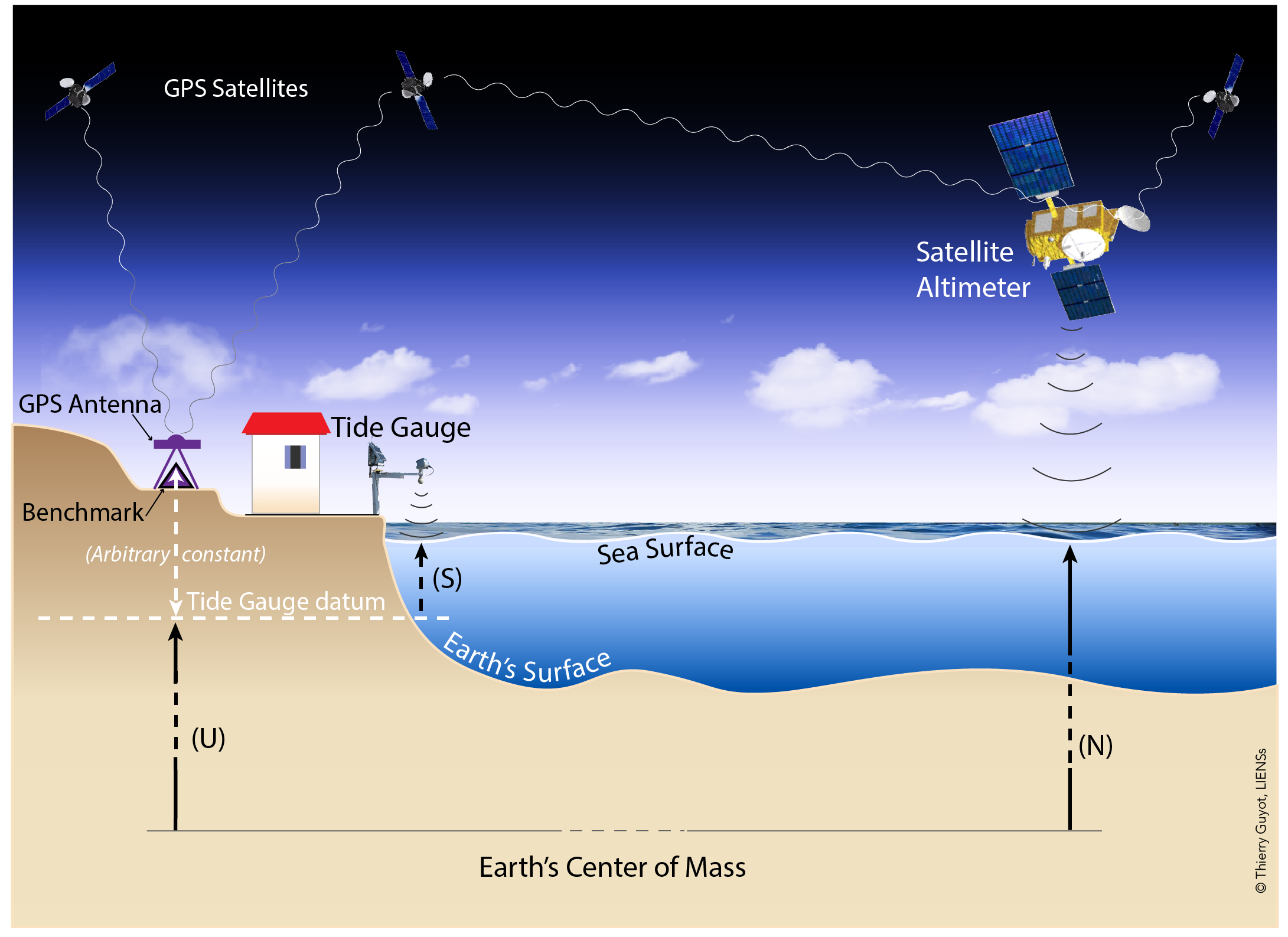
Neither method measures one uniform “height of the ocean.” Sea level varies geographically with circulation, winds, temperature, gravity and other influences. Global mean sea level (GMSL) is a spatial average constructed from observations under a stated set of coverage and processing choices. It describes a global change, not the water level that every coastline experiences.

From a radar pulse to a satellite global mean

An altimeter sends a radar pulse towards the ocean and times its return. To first approximation, half the round-trip travel time multiplied by the speed of light gives the distance from satellite to sea surface. Subtract that distance from the satellite’s precisely determined orbital height, and you have an estimate of geocentric sea-surface height.

Watch the short portions of Rising Seas More Accurately Measured From Space from VideoFromSpace for the instrument principle and the reason successive missions need to be joined carefully.

The apparent simplicity of that subtraction hides much of the work. Researchers need an accurate orbit; corrections for effects on the radar signal as it passes through the atmosphere; and treatment of ocean tides, atmospheric effects and other variations that are not the signal being estimated. They also have to monitor changes in instrument calibration across missions. A small persistent offset between two missions can resemble a step in sea level; a changing calibration error can resemble a trend or acceleration.

The Sea Level Research Group FAQ describes the construction of sea-surface height anomalies: heights are compared with a mean sea surface, relevant time-varying effects are treated, and observations are combined into an area-weighted mean for each repeat cycle.

The satellite record provides far better open-ocean spatial coverage than coastal gauges, but it is not literally complete coverage of every ocean location. The FAQ notes a latitude limit of about $66^{\circ }$ north and south for the missions it discusses. Measurements near coasts are also more difficult: land can interfere with the radar return and with atmospheric corrections. A GMSL estimate therefore needs a defined observational footprint and choices about poorly sampled areas.

If an analysis divides the observed ocean into cells, the averaging principle is

where $A_i$ is cell $i$’s ocean area and $\Delta h_{i,t}$ its estimated height anomaly. Area weighting prevents a densely sampled region from counting simply because it contains more observations. It does not eliminate errors in the measurements or supply information about unobserved regions.

What the coastal record adds

A tide gauge continuously or frequently measures water level against a local benchmark. Instruments have changed—from mechanical floats to pressure, acoustic and radar systems—but the benchmark and its documented stability remain central. Long gauge records extend much further back than the satellite era and observe the coastline directly.

Vertical land motion is a leading source of difference between a gauge trend and a geocentric sea-surface trend. Causes include local subsidence, tectonic movement and glacial isostatic adjustment (GIA)—the continuing response of the solid Earth to the removal of ancient ice sheets. GPS installed at or near a gauge can help estimate land motion. But a GPS trend measured recently need not describe the land’s movement over an entire century-long gauge record, and land motion can differ even between nearby sites.

Land motion is not the only issue. Winds and changing ocean circulation redistribute water, so a region’s sea level can rise faster or slower than the global mean for years or decades. Atmospheric pressure affects local water level through the inverted barometer effect. Tides, storms and other short-term fluctuations must likewise be handled according to the timescale and question. Processing these influences is not an attempt to make every coast follow the global curve: persistent regional differences are physically real and matter locally.

Building a historical global record

The historical gauge network is an awkward sample for estimating a global ocean-area mean. Gauges sit on coasts and islands, not evenly across the ocean. Their geographical distribution and number have changed over time, and different stations use different local benchmarks. A raw average of their reported heights has no meaningful common datum. Converting records to changes or anomalies addresses the differing height origins, but it does not remove uneven sampling or land-motion effects.

The Climate Data Guide explains why historical reconstructions use statistical methods—and sometimes spatial information learned during the satellite era—to estimate change in regions that gauges did not observe.

This creates a useful division of labour. Satellites provide a relatively consistent, near-global view of recent decades. Gauges provide the longer historical context and direct evidence at coasts; they also help check satellite measurements for drift where the records overlap. Reconstructions gain reach by combining information, but their uncertainty must reflect how well the observed coasts represent unobserved ocean regions. A trend from a historical gauge reconstruction and one from a satellite-era product should not be compared without checking their periods, spatial definitions and adjustments.

One adjustment especially illustrates why the definition of the target quantity matters. GIA changes not only some coastal land elevations but also the shape and capacity of the ocean basins. Some satellite GMSL products add a model-based GIA adjustment so that their reported rate better represents ocean-volume change associated with water mass and density, rather than geocentric sea-surface change alone. The FAQ gives an illustrative correction of about $0.3$ mm/year. This is not a correction to be applied indiscriminately to every published number; check the product’s stated convention.

Reading a reported rise—and its uncertainty

The lower panel of the following figure shows one processed satellite GMSL series from January 1993 through December 2021. The red record fluctuates, while its dashed quadratic fit bends upward. The figure reports a trend of $3.3\pm 0.3$ mm/year and an acceleration of $0.12\pm 0.05$ mm/year squared for that analysis and period. Do not transfer those uncertainties to other products or periods, or assume a confidence level that the figure does not state.

A quadratic summary can be written as

where ${\tau }_t$ is time in years, $v$ is a rate at the chosen time origin, and $a$ is an acceleration. The fitted rate at a particular time is $v+a{\tau }_t$. Changing the time origin changes the interpretation of $v$, but not $a$. The figure’s stated trend is best read as its reported summary for the specified interval unless the accompanying study defines its coefficient convention more precisely.

Panel (a) deserves as much attention as the smooth fitted curve. It compares two versions of a processed record and shows that revisions are not necessarily one constant vertical shift. A constant offset would leave a fitted trend unchanged; a difference that changes over time can affect the trend or acceleration. The panel does not, on its own, establish which version is correct or isolate the reason for the revision.

For a careful uncertainty assessment, separate at least three issues:

• Measurement and calibration: orbit determination, radar and atmospheric corrections, instrument drift, and offsets when missions are joined.
• Coverage and geophysical adjustment: unsampled high latitudes or difficult coastal regions; gauge-network clustering; land-motion estimates; and the chosen GIA convention.
• Inference from a finite record: ocean variability, correlated residuals, selected start and end dates, and whether a straight line or quadratic is an adequate summary.

Your previous lesson’s point about autocorrelation applies here too: many closely spaced sea-level observations do not amount to equally many independent pieces of evidence about acceleration. A small formal standard error from a curve fit would not, by itself, capture uncertainty shared across years by a calibration drift or a geophysical correction. Conversely, visible fluctuations around a rising curve do not make the long-term rise disappear. The appropriate conclusion depends on the estimated quantity, the data-processing choices and uncertainty analyses that test their sensitivity.

Conclusion

Satellite altimetry estimates geocentric sea-surface change over much of the ocean and supplies the strongest spatial view of recent GMSL. Tide gauges measure relative sea level at coasts, provide longer records and help validate the satellite series. Turning either into a global trend requires explicit choices about reference frames, coverage, calibration and adjustments; interpreting an acceleration additionally requires attention to time-correlated variability and systematic errors.

Next, the course examines glacier mass balance. There, too, different instruments observe different physical quantities, and understanding their uncertainties is essential before combining them into a climate-change assessment.