Convexity in Optimization: Definitions and Properties

Recommended resources

The freely available resources this lesson will direct you to.

Hello! Let's continue our exploration of optimization theory.

Introduction

In our last lesson, we developed a powerful tool: the second derivative test using the Hessian matrix to classify critical points as local minima, local maxima, or saddle points. We noted a crucial limitation: this test only provides information about the local behavior of a function. In machine learning, we're typically searching for a global minimum of a loss function, and a purely local test doesn't protect us from getting stuck in a "valley" that isn't the lowest point overall.

This lesson introduces the concept that provides the solution: convexity. Functions that are convex have a special "bowl-like" shape that guarantees any local minimum is also a global minimum. This property is the theoretical bedrock for why many optimization algorithms in machine learning are guaranteed to work.

Today's learning outcome is to define convex sets and convex functions, and state their key properties in optimization. We will build the formal mathematical foundation needed to understand and work with these crucial concepts.

Part 1: Convex Sets

Before we can define a convex function, we must first understand what a convex set is, as the domain of a convex function must itself be a convex set.

The core idea is simple: a set is convex if, for any two points you pick within the set, the straight line segment connecting them is also entirely contained within the set.

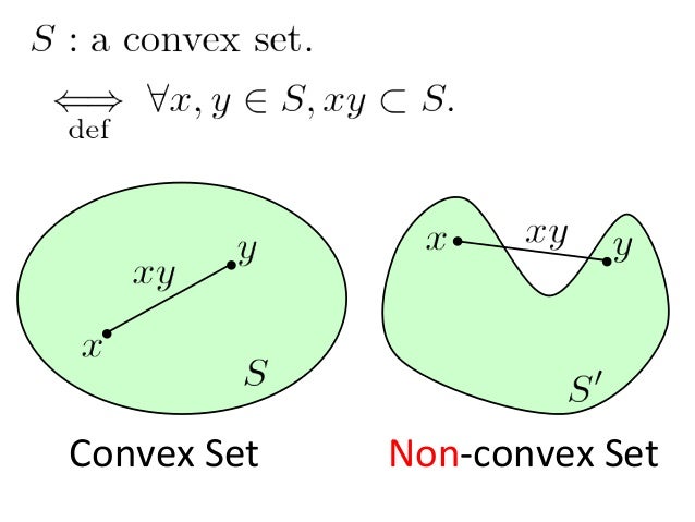
Convex Set Definition and Illustration — This image provides the formal definition of a convex set alongside a clear visual contrast. In the convex set (left), any line segment between two points stays inside the set. In the non-convex set (right), it's possible to draw a line segment that leaves the set.

Formal Definition

A set $C \subseteq R^{n}$ is convex if for any $x_{1}, x_{2} \in C$ and any $θ$ with $0 \leq θ \leq 1$ , we have:

θ x_{1} + (1 - θ) x_{2} \in C

The point $θ x_{1} + (1 - θ) x_{2}$ is called a convex combination of $x_{1}$ and $x_{2}$ . As $θ$ varies from 0 to 1, this expression traces the line segment from $x_{2}$ to $x_{1}$ .

To build a strong intuition for convex sets and see the common examples that appear throughout optimization, please watch the following video segments.

Stanford EE364A Convex Optimization I Stephen Boyd I 2023 I Lecture 2

This video from Stephen Boyd's renowned Stanford course on Convex Optimization will introduce the fundamental concepts of affine and convex combinations and then use them to define several important examples of convex sets.

Please watch the following two segments: From 08:04 to 12:34, focusing on the geometric interpretation of affine and convex combinations. From 24:50 to 32:27, which describes common examples of convex sets like hyperplanes, half-spaces, Euclidean balls, and ellipsoids. You will encounter these sets frequently when formulating ML problems.

As the video explains, some key examples of convex sets include:

Hyperplanes and Half-spaces: The solution set to $a^{T} x = b$ (hyperplane) or $a^{T} x \leq b$ (half-space).
Euclidean balls and Ellipsoids: The set of points within a certain distance of a center point.
Polyhedra: The intersection of a finite number of half-spaces, i.e., the solution set to $A x \leq b$ .
The Positive Semidefinite Cone: The set of all symmetric positive semidefinite matrices, which you'll recall from our last lesson on Hessians.

A crucial property, which we will see again with convex functions, is that intersection preserves convexity. If you take the intersection of any number of convex sets, the resulting set is also convex.

Part 2: Convex Functions

With the definition of a convex set in hand, we can now define a convex function. Geometrically, a function is convex if the line segment connecting any two points on its graph lies on or above the graph.

Definition of Convex Functions — This image from the book \"Convex Optimization\" shows the defining characteristic of a convex function. The chord connecting (x, f(x)) and (y, f(y)) is always above the function graph between those points.

Formal Definition

A function $f : R^{n} \to R$ is convex if its domain, dom(f), is a convex set and for all $x, y \in dom (f)$ and any $θ$ with $0 \leq θ \leq 1$ , we have:

f (θ x + (1 - θ) y) \leq θ f (x) + (1 - θ) f (y)

Notice the inequality: the value of the function at a convex combination of points is less than or equal to the convex combination of the function's values at those points.

A function $f$ is concave if $- f$ is convex. A function is strictly convex if the inequality is strict ( $<$ ) for $0 < θ < 1$ and $x \neq = y$ .

Connection to Convex Sets: The Epigraph

There is a beautiful and fundamental connection between convex functions and convex sets. The epigraph of a function $f$ , denoted epi(f), is the set of points lying on or above its graph:

epi (f) = {(x, t) ∣ x \in dom (f), t \geq f (x)}

A function $f$ is convex if and only if its epigraph epi(f) is a convex set. This provides a direct bridge between the two concepts.

Key Properties of Convex Functions

While the definition is fundamental, it's not always easy to apply directly. In practice, we rely on a set of powerful properties or conditions to verify convexity. These are the tools you will use most often.

The following video discusses the most important of these properties.

Lecture 3 | Convex Optimization I (Stanford)

Let's return to Stephen Boyd's lecture. This segment is one of the most important in the course, as it explains the first and second-order conditions for convexity, which directly relate to the calculus concepts we've already covered.

Please watch from 10:20 to 12:45 to see the formal definition. Then, watch carefully from 31:22 to 40:58. This part covers the first-order and second-order conditions. Pay special attention to the interpretation of the first-order condition as a global underestimator—this is the key to why convex optimization works.

Let's summarize these two crucial conditions. For a function $f$ that is differentiable:

First-Order Condition: $f$ is convex if and only if its domain is convex and for all $x, y$ in its domain:
$f (y) \geq f (x) + \nabla f (x)^{T} (y - x)$
This is a profound result. The right-hand side is the first-order Taylor approximation of $f$ at $x$ . This inequality states that for a convex function, the tangent hyperplane at any point is a global underestimator of the function. This means that local information (the gradient at a point) gives us global information (a bound on the entire function).
Second-Order Condition: Assume $f$ is twice differentiable. Then $f$ is convex if and only if its domain is convex and its Hessian matrix is positive semidefinite everywhere in its domain:
$\nabla^{2} f (x) ⪰ 0 for all x \in dom (f)$
This provides a direct link to our previous lesson. The "upward curvature" of a convex function is captured by the positive semidefiniteness of its Hessian. This is often the easiest way to check for convexity for smooth functions.

Test your understanding!

Consider a general quadratic function $f (x) = \frac{1}{2} x^{T} P x + q^{T} x + r$ , where $P$ is a symmetric $n \times n$ matrix.

Using the second-order condition for convexity, what property must the matrix $P$ have for $f (x)$ to be convex?

Show answer

First, we need to find the Hessian of $f (x)$ . The gradient is $\nabla f (x) = P x + q$ .
The Hessian is the matrix of second partial derivatives, which is simply $\nabla^{2} f (x) = P$ .

According to the second-order condition, a twice-differentiable function is convex if and only if its Hessian is positive semidefinite.
Therefore, for $f (x)$ to be convex, the matrix $P$ must be positive semidefinite ( $P ⪰ 0$ ).

This is a classic and very important result, especially for linear regression, where the least squares cost function is a quadratic of this form.

Building Convex Functions: A Calculus of Convexity

Much like you can build complex differentiable functions from simpler ones (sums, products, chains), you can also build complex convex functions. This is often how convexity is established in practice for complicated ML loss functions.

Lecture 3 | Convex Optimization I (Stanford)

This final video segment introduces operations that preserve convexity. Understanding this "calculus" of convexity is a powerful skill for verifying that a complex function can be optimized effectively.

Watch from 57:24 to 01:04:15. Focus on these key preserving operations: Non-negative weighted sum: sum(w_i * f_i(x)) Composition with an affine function: f(Ax + b) Pointwise maximum: max(f_1(x), f_2(x), ...)

Key operations that preserve convexity:

Non-negative weighted sum: If $f_{1}, \dots, f_{k}$ are convex and $w_{1}, \dots, w_{k} \geq 0$ , then $f (x) = \sum_{i = 1}^{k} w_{i} f_{i} (x)$ is convex.
Composition with an affine function: If $f$ is convex, then $g (x) = f (A x + b)$ is convex.
Pointwise maximum: If $f_{1}, \dots, f_{k}$ are convex, then $f (x) = max (f_{1} (x), \dots, f_{k} (x))$ is convex. This is very important for many modern ML loss functions (e.g., the hinge loss used in SVMs).

Conclusion

This lesson has been dense with definitions, but these concepts are the absolute foundation of modern optimization theory.

Key Takeaways:

A convex set contains the line segment between any two of its points.
A convex function is one where the line segment between any two points on its graph lies on or above the graph. Formally, a function is convex iff its epigraph is a convex set.
For differentiable functions, convexity has two crucial characterizations:
1. First-Order: The tangent hyperplane is a global underestimator.
2. Second-Order: The Hessian matrix is positive semidefinite everywhere.
Convexity is preserved under key operations like non-negative sums, affine composition, and pointwise maximum, allowing us to prove that complex functions are convex.

Preview of the Next Lesson:
We have laid all the necessary groundwork. Now we can prove the theorem that makes all this theory so powerful. In the next lesson, we will use the first-order condition for convexity to formally prove that for a convex function, any local minimum is also a global minimum. This result is what allows us to be confident in the solutions found by algorithms like gradient descent for a vast class of machine learning models.