Classifying Critical Points with the Hessian Matrix

Hello! Let's dive into the next crucial topic in our journey through optimization theory.

Introduction

In our last lesson, we established how to construct a second-order Taylor approximation for a multivariable function $f(\mathbf{x})$ around a point $\mathbf{a}$:

We previewed that this approximation becomes particularly powerful at critical points, where the gradient $\nabla f(\mathbf{a})$ is the zero vector. At such points, the linear term vanishes, and the local behavior of the function—whether it curves upwards like a valley, downwards like a hilltop, or both like a saddle—is determined entirely by the quadratic term involving the Hessian matrix, $H_f(\mathbf{a})$.

Today, we will formalize this idea. Our learning outcome is to identify critical points of a function and use the Hessian matrix to classify them as local minima, maxima, or saddle points. This is the multivariable equivalent of the second derivative test from single-variable calculus and is a cornerstone of optimization in machine learning.

Step 1: Finding Critical Points

First, let's formally define our terms.

• A point $\mathbf{a}$ is a local minimum if $f(\mathbf{a})\le f(\mathbf{x})$ for all $\mathbf{x}$ in a small neighborhood around $\mathbf{a}$.
• A point $\mathbf{a}$ is a local maximum if $f(\mathbf{a})\ge f(\mathbf{x})$ for all $\mathbf{x}$ in a small neighborhood around $\mathbf{a}$.
• A local extremum is a point that is either a local minimum or a local maximum.

A critical point (also called a stationary point) is a point $\mathbf{a}$ in the interior of the function's domain where the gradient is zero: $\nabla f(\mathbf{a})=0$.

A zero gradient is a necessary condition for a point to be a local extremum. Intuitively, if the gradient were non-zero at a point $\mathbf{a}$, it would point in the direction of steepest ascent. We could take a small step in that direction to find a higher function value, or a small step in the opposite direction to find a lower value. Therefore, $\mathbf{a}$ could not be a local extremum. The only points that can be local extrema are those where the tangent plane is flat.

To find critical points, we must therefore solve the system of equations that arises from setting each partial derivative to zero:

This often results in a system of non-linear equations, which can be challenging to solve.

Step 2: Classifying Critical Points with the Hessian

Finding a critical point only tells us the function's surface is momentarily flat. It doesn't tell us what happens next. Is it the bottom of a bowl (minimum), the top of a hill (maximum), or a mountain pass (saddle point)?

As we saw in the Taylor expansion, this is governed by the quadratic form $\frac{1}{2}{\mathbf{h}}^{T}H\mathbf{h}$, where $\mathbf{h}$ is a small displacement vector and $H$ is the Hessian at the critical point. The sign of this term for different directions $\mathbf{h}$ tells us how the function curves.

Definiteness of the Hessian Matrix

The video correctly points out that classifying a critical point comes down to determining if the Hessian matrix is "positive" or "negative" in some sense. This "sign" of a symmetric matrix is called its definiteness. This is a concept from linear algebra that is deeply connected to the signs of the matrix's eigenvalues.

To summarize the key theorem from the reading: for a symmetric matrix $H$ (and the Hessian is always symmetric for functions you'll encounter in ML):

• $H$ is positive definite $⟺$ all of its eigenvalues are positive (${\lambda }_i>0$).
  • This means ${\mathbf{h}}^{T}H\mathbf{h}>0$ for all non-zero vectors $\mathbf{h}$. Geometrically, the function curves upwards in every direction from the critical point.
• $H$ is negative definite $⟺$ all of its eigenvalues are negative (${\lambda }_i<0$).
  • This means ${\mathbf{h}}^{T}H\mathbf{h}<0$ for all non-zero vectors $\mathbf{h}$. Geometrically, the function curves downwards in every direction.
• $H$ is indefinite $⟺$ it has at least one positive and at least one negative eigenvalue.
  • This means ${\mathbf{h}}^{T}H\mathbf{h}$ is positive for some directions $\mathbf{h}$ and negative for others. Geometrically, the function curves up in some directions and down in others.
• If any eigenvalue is zero and the others are all non-negative (or all non-positive), the matrix is semidefinite.

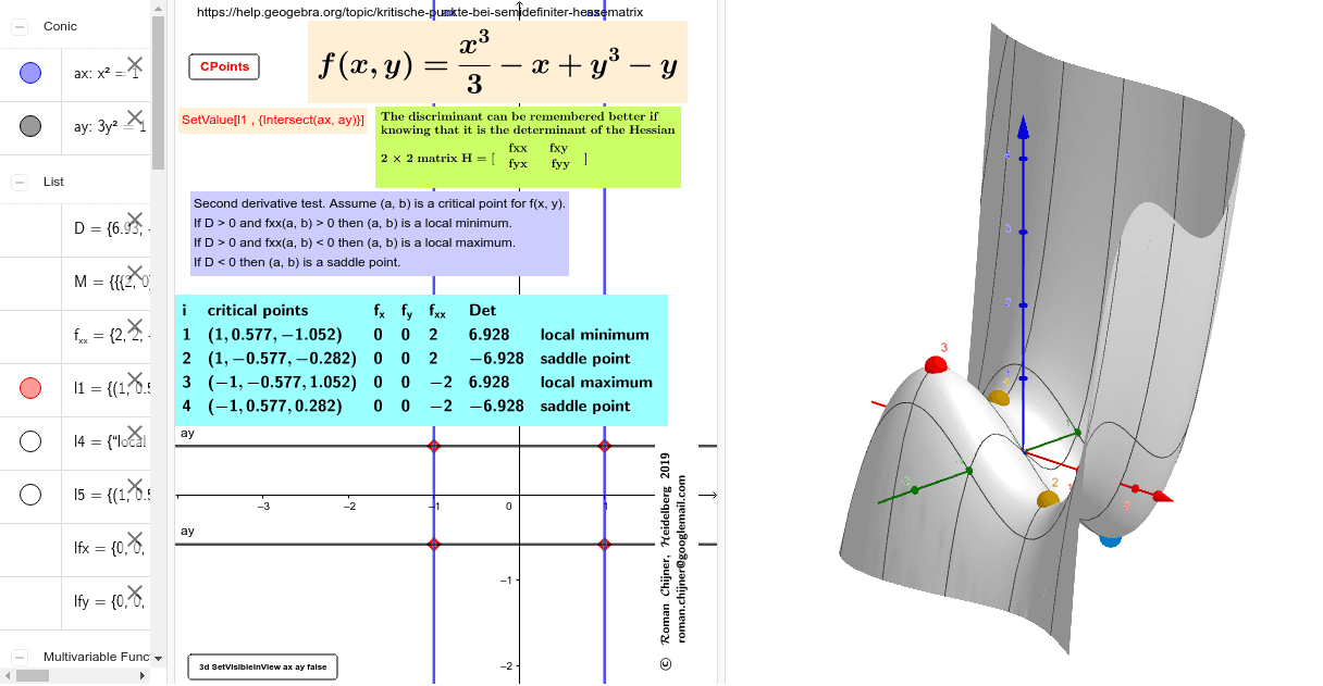
The Second Derivative Test

We can now state the full second derivative test for a $C^2$ function $f$ at a critical point $\mathbf{a}$ where $\nabla f(\mathbf{a})=0$.

1. If $H_f(\mathbf{a})$ is positive definite (all eigenvalues > 0), then $\mathbf{a}$ is a local minimum.
2. If $H_f(\mathbf{a})$ is negative definite (all eigenvalues < 0), then $\mathbf{a}$ is a local maximum.
3. If $H_f(\mathbf{a})$ is indefinite (mixed positive and negative eigenvalues), then $\mathbf{a}$ is a saddle point.
4. If $H_f(\mathbf{a})$ is semidefinite (some eigenvalues are zero, and the rest have the same sign), the test is inconclusive. The point could be a min, max, saddle, or something else entirely (like the flat bottom of a trough).

Step 3: A Complete Worked Example

Let's return to the video example and see the classification step in action. The video uses a common shortcut for 2x2 matrices that avoids directly computing eigenvalues.

Connecting the "D-Test" to Eigenvalues

The video uses a quantity $D=f_{xx}{f}_{yy}-(f_{xy}{)}^2$. You should recognize this as the determinant of the 2x2 Hessian matrix. For a 2x2 matrix, the determinant is the product of the eigenvalues ($\det (H)={\lambda }_1{\lambda }_2$), and the trace is the sum of the eigenvalues ($\text{tr}(H)=f_{xx}+f_{yy}={\lambda }_1+{\lambda }_2$).

This provides the rigorous justification for the "D-test":

• If $\det (H)>0$, then ${\lambda }_1$ and ${\lambda }_2$ have the same sign. The sign is determined by their sum, $\text{tr}(H)$. If $f_{xx}>0$, the trace must be positive, so both eigenvalues are positive (local min). If $f_{xx}<0$, the trace must be negative, so both eigenvalues are negative (local max).
• If $\det (H)<0$, then ${\lambda }_1$ and ${\lambda }_2$ have opposite signs. The Hessian is indefinite (saddle point).
• If $\det (H)=0$, at least one eigenvalue is zero. The Hessian is semidefinite, and the test is inconclusive.

While this shortcut is handy for 2x2 cases, for higher dimensions (which are common in machine learning), you must rely on computing the eigenvalues to determine the definiteness of the Hessian.

Conclusion

Today, we built a complete framework for analyzing the local behavior of multivariable functions, a critical skill for understanding machine learning optimization.

Key Takeaways:

• Critical points are found by solving $\nabla f(\mathbf{x})=0$. They are necessary candidates for local extrema.
• The Hessian matrix at a critical point describes the local curvature of the function.
• The definiteness of the Hessian (positive definite, negative definite, or indefinite) determines the nature of the critical point.
• The definiteness is determined by the signs of the Hessian's eigenvalues. This is the multivariable second derivative test.
  • All ${\lambda }_i>0$ $⟹$ Local Minimum
  • All ${\lambda }_i<0$ $⟹$ Local Maximum
  • Mixed ${\lambda }_i$ signs $⟹$ Saddle Point

Preview of the Next Lesson:
We have focused on characterizing local minima. However, in machine learning, we are often interested in finding the global minimum of a loss function. A major challenge is that an algorithm might get stuck in a local minimum that isn't the global one. In our next lesson, we will introduce the powerful concepts of convex sets and convex functions. For convex functions, the landscape is shaped like a single bowl, which guarantees that any local minimum is also a global minimum. This property is fundamental to proving why optimization works for many important ML models.