Smoothness and Strong Convexity

Recommended resources

The freely available resources this lesson will direct you to.

Hello! Let's build on our practical work with gradient descent by exploring the theoretical properties that govern its performance.

Introduction

In our last lesson, you successfully implemented the gradient descent algorithm and experimented with the learning rate, $η$ . You observed firsthand that the algorithm's convergence—or divergence—is highly sensitive to both $η$ and the shape of the function being minimized. This empirical understanding is crucial, but as you requested, our goal is to build a rigorous theoretical foundation.

Today's lesson addresses the learning outcome: Define smoothness (Lipschitz continuity) and strong convexity of a function. These two properties provide a formal, mathematical language to describe the "shape" or "curvature" of a function. Understanding them is the critical prerequisite for analyzing why gradient descent converges and how quickly it does so. We will move from trial-and-error to formal analysis, setting the stage to derive concrete convergence rates.

Why These Properties Matter

Before diving into formal definitions, it's helpful to build intuition. When we run gradient descent, we face two potential problems related to curvature:

The gradient changes too quickly: If the function's curvature is very sharp and changes erratically, a step we take based on the gradient at one point might land us in a region with a completely different gradient, causing us to "overshoot" the minimum wildly. We need a way to control how fast the gradient can change. This leads to the concept of smoothness.
The function is too flat: If the function is very flat around the minimum (like a wide, shallow bowl), the gradient will be very close to zero even when we are still far from the true minimum. This causes the algorithm to take tiny, inefficient steps, slowing convergence to a crawl. We need the function to be "curved enough" to guarantee progress. This leads to the concept of strong convexity.

The following video provides an excellent introduction to this motivation by comparing a quadratic function (which behaves well) to the absolute value function (which presents challenges for gradient descent).

3.2 Smooth and Strongly Convex Functions

Watch the introductory part of this video from Constantine Caramanis to get a feel for the practical implications of these properties.

Watch the segment from 00:08 to 05:22. The speaker discusses the different behaviors of gradient descent on a quadratic function versus an absolute value function. Pay attention to his description of the 'self-tuning' property and how the gradient's magnitude behaves far from the solution. These are the intuitions we are about to formalize.

Part 1: Smoothness (Lipschitz Continuity of the Gradient)

Smoothness formalizes the idea that the gradient does not change too rapidly. A function is considered smooth if its gradient is Lipschitz continuous.

Formal Definition

A differentiable function $f : R^{n} \to R$ is called $L$ -smooth if its gradient $\nabla f$ is Lipschitz continuous with constant $L > 0$ . This means that for any two points $x, y$ in its domain:

∥\nabla f (x) - \nabla f (y) ∥_{2} \leq L ∥ x - y ∥_{2}

Here, $∥ \cdot ∥_{2}$ is the standard Euclidean norm. This inequality states that the distance between the gradient vectors at two points is bounded by $L$ times the distance between the points themselves. The constant $L$ limits how much the gradient can change.

The Consequence: A Quadratic Upper Bound

The most important consequence of $L$ -smoothness for optimization is that it implies the function is globally upper-bounded by a quadratic. For any $x, y$ :

f (y) \leq f (x) + \nabla f (x)^{T} (y - x) + \frac{L}{2} ∥ y - x ∥_{2}^{2}

Notice the first two terms on the right, $f (x) + \nabla f (x)^{T} (y - x)$ , form the first-order Taylor approximation (the tangent plane) of $f$ at $x$ . Smoothness guarantees that the function $f (y)$ cannot grow faster than this tangent plane plus a simple quadratic term. This prevents the function from curving upwards too sharply.

To understand how this crucial inequality is derived from the definition of smoothness, please study the following resources. The video provides a detailed walkthrough, while the PDF offers a concise, formal proof.

3.2 Smooth and Strongly Convex Functions

This segment of the video provides a rigorous derivation of the quadratic upper bound from the definition of smoothness.

Watch from 08:02 to 19:53. The presenter defines a helper function g(x) and proves it is convex. He then uses the first-order condition for convexity of g(x) to derive the final inequality. Follow each step of the algebraic manipulation carefully.

1. Gradient method

For a more compact reference, review the following lecture notes from a UCLA optimization course by Vandenberghe et al. They demonstrate the equivalence between the Lipschitz condition and the quadratic upper bound.

Read pages 1-10 to 1-12. Page 1-10 gives the formal definition of a Lipschitz continuous gradient. Page 1-11 states the quadratic upper bound, and page 1-12 provides the proof of equivalence. This proof uses a slightly different but equally valid method involving integration along the line segment between x and y.

Connection to the Hessian

For a twice-differentiable function, there is a very direct way to determine if it is $L$ -smooth. The condition is equivalent to the eigenvalues of its Hessian matrix $\nabla^{2} f (x)$ being bounded above by $L$ for all $x$ . Using matrix notation, this is written as:

\nabla^{2} f (x) ⪯ L I

where $I$ is the identity matrix and the $⪯$ symbol means that the matrix $L I - \nabla^{2} f (x)$ is positive semidefinite. This gives us a practical tool to find the smoothness constant for many functions. For example, for a quadratic function $f (x) = \frac{1}{2} x^{T} Ax$ , the Hessian is the constant matrix $A$ , so its smoothness constant $L$ is simply the largest eigenvalue of $A$ .

Test your understanding!

Consider the one-dimensional function $f (x) = \frac{1}{4} x^{4}$ .

Is this function smooth?
If so, can we find a single, global smoothness constant $L$ that holds for all $x \in R$ ? Why or why not?

Show answer

Yes, the function is smooth. Its gradient is $f^{'} (x) = x^{3}$ , and its second derivative is $f^{''} (x) = 3 x^{2}$ . Both are continuous functions.
No, we cannot find a single, global smoothness constant $L$ . The condition for smoothness in 1D for a twice-differentiable function is $f^{''} (x) \leq L$ . For our function, this means $3 x^{2} \leq L$ . This inequality cannot hold for all $x \in R$ with a finite constant $L$ , because $3 x^{2}$ grows without bound as $∣ x ∣ \to \infty$ . The function is therefore called locally smooth (it has a valid $L$ in any bounded region) but not globally smooth. This is an important distinction in optimization theory.

Part 2: Strong Convexity

Strong convexity is, as the name suggests, a stronger condition than the standard convexity we have already discussed. It formalizes the notion that a function must be "sufficiently curved" and cannot have flat regions.

Formal Definition

A differentiable function $f$ is $m$ -strongly convex with parameter $m > 0$ if for any two points $x, y$ in its domain, the following inequality holds:

f (y) \geq f (x) + \nabla f (x)^{T} (y - x) + \frac{m}{2} ∥ y - x ∥_{2}^{2}

Compare this to the standard first-order condition for convexity: $f (y) \geq f (x) + \nabla f (x)^{T} (y - x)$ . Strong convexity adds the extra quadratic term $\frac{m}{2} ∥ y - x ∥_{2}^{2}$ , which forces the function to lie strictly above its tangent plane. This provides the desired quadratic lower bound.

The following resources provide the formal definition and derivation.

3.2 Smooth and Strongly Convex Functions

The same video now introduces strong convexity, defining it in a way that directly parallels the discussion on smoothness.

Watch the segment from 23:00 to 27:18. The presenter defines strong convexity by stating that f(x) - (m/2)||x||^2 is a convex function. He then uses this definition to derive the quadratic lower bound inequality shown above. Observe the symmetry in the argument compared to the smoothness section.

3 Smoothness and strong convexity

These lecture notes provide a clear, formal definition of strong convexity and its consequences.

Read section 3.3, "Strong convexity" (page 2). Note the definition using Jensen's inequality (4), and the equivalent condition for differentiable functions (5), which is the quadratic lower bound we are focusing on.

Connection to the Hessian

Similar to smoothness, strong convexity has a direct link to the Hessian for twice-differentiable functions. A function is $m$ -strongly convex if and only if the eigenvalues of its Hessian matrix $\nabla^{2} f (x)$ are all bounded below by $m$ for all $x$ . In matrix notation:

\nabla^{2} f (x) ⪰ m I

This means that the matrix $\nabla^{2} f (x) - m I$ must be positive semidefinite. For our quadratic example $f (x) = \frac{1}{2} x^{T} Ax$ (with $A$ being symmetric positive definite), the strong convexity constant $m$ is the smallest eigenvalue of $A$ .

The "Sandwich" Property and Its Importance

Now, let's put everything together. If a function $f$ is both $L$ -smooth and $m$ -strongly convex, it is confined between a quadratic lower bound and a quadratic upper bound:

Quadratic Lower Bound f (x) + \nabla f (x)^{T} (y - x) + \frac{m}{2} ∥ y - x ∥_{2}^{2} \leq f (y) \leq Quadratic Upper Bound f (x) + \nabla f (x)^{T} (y - x) + \frac{L}{2} ∥ y - x ∥_{2}^{2}

This "sandwiching" of the function between two quadratics is the single most important result of this lesson.

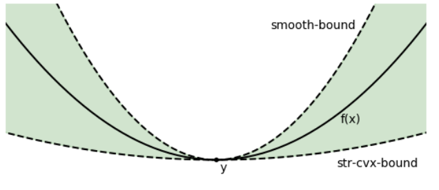
Visualizing Smoothness and Strong Convexity — This image provides a powerful visualization of what we've derived. The function f(x) is constrained to lie within the region between the parabolic lower bound from strong convexity (str-cvx-bound) and the parabolic upper bound from smoothness (smooth-bound).

The ratio $κ = L / m$ is called the condition number of the function. It measures how "well-behaved" the function is for optimization.

If $κ$ is close to 1, then $L \approx m$ , meaning the function's curvature is very uniform. It behaves almost like a perfect sphere, which is ideal for gradient descent.
If $κ$ is very large, the function is ill-conditioned. This means it's very steep in some directions and very flat in others (like the elongated bowl from our previous lesson's implementation, $f (x_{1}, x_{2}) = x_{1}^{2} + 5 x_{2}^{2}$ ). This is where gradient descent can struggle.

This condition number $κ$ will be the central quantity when we analyze the convergence rate in our next lesson.

Test your understanding!

Let's return to the function from the previous lesson: $f (x_{1}, x_{2}) = x_{1}^{2} + 5 x_{2}^{2}$ .

Calculate the Hessian matrix $\nabla^{2} f (x)$ .
What are its eigenvalues?
Based on the eigenvalues, what are the smoothness constant $L$ and the strong convexity constant $m$ for this function?
What is the condition number $κ$ ?

Show answer

First, we find the gradient: $\nabla f (x) = [2 x_{1} 10 x_{2}]$ . The Hessian is the matrix of second partial derivatives: $\nabla^{2} f (x) = [\frac{\partial ^{2} f}{\partial x _{1}^{2}} \frac{\partial ^{2} f}{\partial x _{2} \partial x _{1}} \frac{\partial ^{2} f}{\partial x _{1} \partial x _{2}} \frac{\partial ^{2} f}{\partial x _{2}^{2}}] = [20010]$
Since the Hessian is a diagonal matrix, its eigenvalues are the diagonal entries: $λ_{1} = 2$ and $λ_{2} = 10$ .
The smoothness constant $L$ is the largest eigenvalue: $L = 10$ . The strong convexity constant $m$ is the smallest eigenvalue: $m = 2$ .
The condition number is $κ = L / m = 10/2 = 5$ .

Conclusion

In this lesson, we have established the formal definitions and implications of two fundamental properties in optimization theory.

Key Takeaways:

L-smoothness (Lipschitz Gradient): Limits how fast the gradient can change. It provides a quadratic upper bound on the function, ensuring it doesn't curve "too sharply." For twice-differentiable functions, it's equivalent to $λ_{m a x} (\nabla^{2} f) \leq L$ .
m-strong convexity: Requires the function to be sufficiently curved everywhere. It provides a quadratic lower bound, ensuring the function isn't "too flat." For twice-differentiable functions, it's equivalent to $λ_{m i n} (\nabla^{2} f) \geq m$ .
The Sandwich: A function that is both L-smooth and m-strongly convex is bounded between two quadratics. This property is the key to proving convergence guarantees for gradient descent.
Condition Number: The ratio $κ = L / m$ quantifies how "well-behaved" the function is. A large $κ$ indicates an ill-conditioned problem.

Preview of the Next Lesson:
We are now fully equipped to analyze the convergence of gradient descent with mathematical rigor. In the next lesson, we will use the quadratic upper and lower bounds derived today to prove that for an $L$ -smooth and $m$ -strongly convex function, gradient descent converges at a linear rate. We will derive an explicit formula that shows exactly how the error decreases at each iteration as a function of $L$ and $m$ .