Implementing Gradient Descent

Hello! Let's dive into the practical side of optimization.

Introduction

In our previous lesson, we rigorously derived the gradient descent update rule from first principles:

$${\mathbf{x}}_{k+1}={\mathbf{x}}_k-\eta \nabla f({\mathbf{x}}_k)$$

We established that moving in the direction of the negative gradient, $-\nabla f(\mathbf{x})$, is the path of steepest descent, providing the theoretical justification for this algorithm.

Today, we will translate this mathematical theory into practice. Your goal for this lesson is to implement the gradient descent algorithm to find the minimum of a simple convex function. This will connect the abstract derivations directly with your Python programming experience. You'll write the code to make a point "roll downhill" on a function's surface to find its minimum, solidifying your understanding of this fundamental optimization workhorse.

---

Part 1: Defining the Optimization Problem

Before we write any code, we must first define the function we want to minimize. As per the learning outcome, we'll use a simple, multivariable convex function. This ensures that the local minimum we find is also the global minimum, a property you proved in a prior lesson.

Let's choose the following quadratic function:

$$f(x_1,x_2)=x_1^2+5x_2^2$$

This function is a paraboloid, but stretched more steeply along the $x_2$-axis. Its minimum is clearly at $(0,0)$.

The first step in implementing gradient descent is always to compute the gradient of the objective function. Given your calculus background, you can quickly find the partial derivatives:

• $\frac{\partial f}{\partial x_1}=2x_1$
• $\frac{\partial f}{\partial x_2}=10x_2$

So, the gradient vector is:

$$\nabla f(\mathbf{x})=\left[\begin{array}{c}2x_1\\ 10x_2\end{array}\right]$$

With $f(\mathbf{x})$ and $\nabla f(\mathbf{x})$ defined, we have all the mathematical components needed to implement our algorithm.

---

Part 2: Implementing Gradient Descent in Python

Now, we will write the Python code to perform the optimization. We will use NumPy for numerical operations and Matplotlib for visualization, tools you are already familiar with.

The following video provides an excellent walkthrough of implementing gradient descent from scratch. It starts with a simple 1D case and then moves to a 2D (or 3D surface) case. While the video uses a different, non-convex function for its 2D example, the implementation logic—defining the function, its gradient, and the iterative update loop—is universal.

Now, it's your turn to build it. Using the patterns from the video and the structured approach outlined in the following text, you will implement gradient descent for our specific function, $f(x_1,x_2)=x_1^2+5x_2^2$.

Your Task: Implement Gradient Descent

Follow these steps in a Jupyter Notebook or Python script:

1. Import libraries: numpy and matplotlib.pyplot.
2. Define the functions:
   • f(x): Takes a 2-element NumPy array x and returns $x_1^2+5x_2^2$.
   • grad_f(x): Takes a 2-element NumPy array x and returns the gradient, np.array([2*x[0], 10*x[1]]).
3. Set up the algorithm:
   • Initialize a starting point, e.g., x_current = np.array([10.0, 2.0]).
   • Choose a learning rate, e.g., eta = 0.05.
   • Set the number of iterations, e.g., n_iterations = 100.
   • Create an empty list history to store the position x_current at each iteration.
4. Create the main loop:
   • Loop for n_iterations.
   • In each iteration:
     • Calculate the gradient at the current position: gradient = grad_f(x_current).
     • Update the position using the rule: x_current = x_current - eta * gradient.
     • Append x_current to your history list.
5. Visualize the results:
   • After the loop, you can print the final position x_current to see how close it got to [0, 0].
   • Use matplotlib to create a contour plot of the function and overlay the path taken by the algorithm (from your history list). The resources above contain examples of how to generate these plots.

---

Part 3: The Critical Role of the Learning Rate

In the last lesson, we noted the importance of the step size $\eta$. Now you can see its effect firsthand. A poorly chosen $\eta$ can lead to slow convergence or even cause the algorithm to fail completely.

The video you watched earlier has an excellent segment demonstrating this.

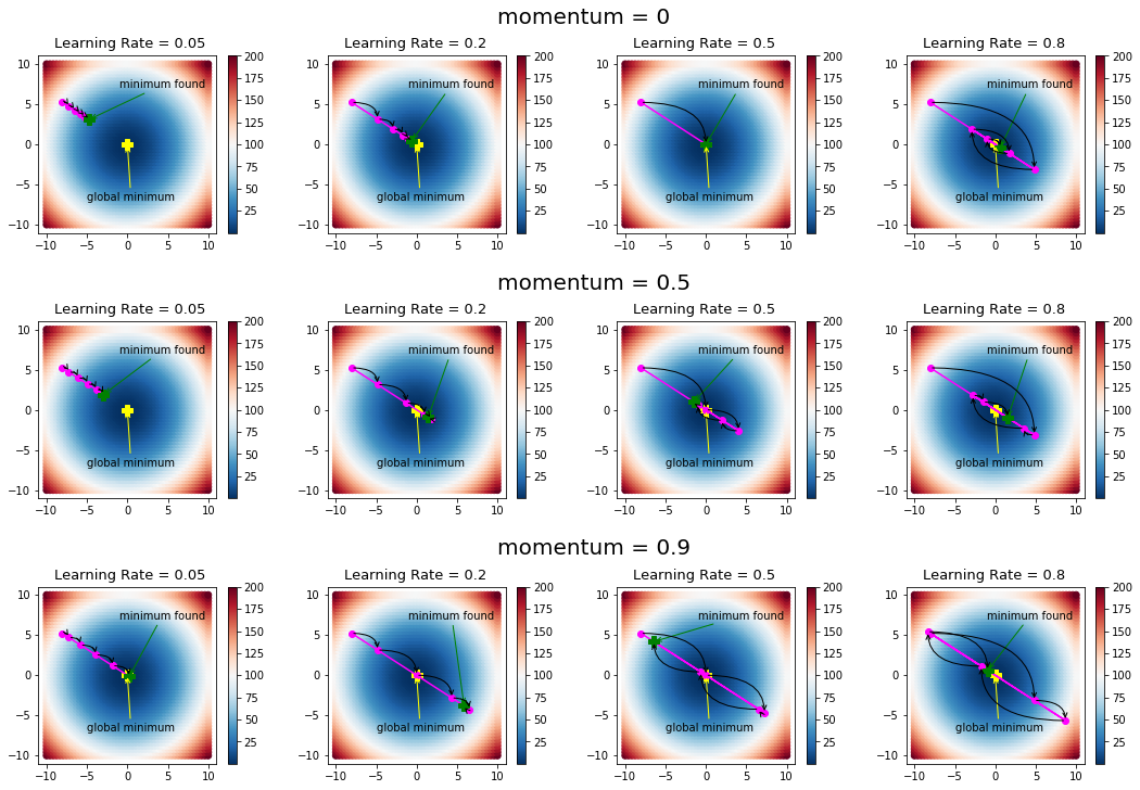
Now, experiment with your own implementation. Run your code with three different learning rates:

• A small learning rate (e.g., eta = 0.001)
• A good learning rate (e.g., eta = 0.05)
• A large learning rate (e.g., eta = 0.19)
• An even larger learning rate (e.g., eta = 0.21)

Visualize the path for each. You will see the behavior change dramatically.

Test your understanding!

Our objective function is $f(x_1,x_2)=x_1^2+5x_2^2$. The gradient is $\nabla f(\mathbf{x})=[2x_1,10x_2{]}^T$. Notice that for the same point $(x_1,x_2)$, the gradient component is larger in the $x_2$ direction.

If you use a learning rate that is slightly too large, in which direction ($x_1$ or $x_2$) would you expect the algorithm to start oscillating or diverging first? Why?

Show answer

You would expect the algorithm to start oscillating or diverging in the $x_2$ direction first.

The update for each component is $x_{k+1}=x_k-\eta \cdot {\text{gradient}}_k$. Since the gradient component for $x_2$ ($10x_2$) is five times larger than for $x_1$ ($2x_1$) at any given point, the step taken in the $x_2$ direction is much larger. This larger step makes it more likely to overshoot the minimum along that axis, leading to oscillation or divergence. This illustrates how the function's curvature (which is steeper along the $x_2$-axis) interacts with the learning rate.

---

Conclusion

Congratulations! You have successfully implemented one of the most fundamental algorithms in machine learning. By translating the mathematical formula into working code, you have bridged the gap between theory and practice.

Key Takeaways:

• Gradient descent is implemented as an iterative loop that repeatedly calculates the gradient and updates the current parameters.
• The essential ingredients are the objective function, its gradient, a starting point, a learning rate, and a number of iterations.
• The learning rate ($\eta$) is a critical hyperparameter. If it's too small, convergence is slow. If it's too large, the algorithm can oscillate or diverge.
• Visualizing the optimization path on a contour plot is a powerful tool for understanding the algorithm's behavior.

Preview of the Next Lesson:
We've built an intuition for how convergence works, but our choice of $\eta$ and the number of iterations was based on trial and error. To be more rigorous, we need to analyze the algorithm's convergence properties mathematically. In the next lesson, we will define two key properties of functions—smoothness and strong convexity—which will allow us to derive formal guarantees on the convergence rate of gradient descent. This will help us answer the question: "How fast does gradient descent find the minimum?"