Comparing Linear and Cosine Noise Schedules via Signal-to-Noise Profiles

Last lesson established that a diffusion timestep is best understood by its noise level, not by its integer index. For a variance-preserving forward process,

$${\mathbf{x}}_t={\alpha }_t{\mathbf{x}}_0+{\sigma }_t\mathbf{ϵ},{\alpha }_t^2+{\sigma }_t^2=1,$$

the relevant diagnostic is

$${\mathrm{SNR}}_t=\frac{{\alpha }_t^2}{{\sigma }_t^2}=\frac{{\bar{\alpha }}_t}{1-{\bar{\alpha }}_t}.$$

This lesson asks a more practical question: how does the choice of noise schedule distribute SNR over the trajectory? We will compare the original DDPM linear schedule with the cosine schedule introduced by Nichol and Dhariwal, and distinguish carefully between “linear in timestep” and “linear in the actual corruption level.”

---

Two meanings of “schedule”

A diffusion schedule can be specified in several equivalent ways:

• Per-step noise variances ${\beta }_t$
• Cumulative retained-signal variance ${\bar{\alpha }}_t$
• Signal and noise amplitudes ${\alpha }_t$ and ${\sigma }_t$
• SNR or log SNR

For comparison, the cumulative form is usually most revealing:

$${\mathbf{x}}_t=\sqrt{{\bar{\alpha }}_t}{\mathbf{x}}_0+\sqrt{1-{\bar{\alpha }}_t}\mathbf{ϵ}.$$

Thus,

$${\alpha }_t=\sqrt{{\bar{\alpha }}_t},{\sigma }_t=\sqrt{1-{\bar{\alpha }}_t}.$$

Here ${\alpha }_t$ denotes the total signal amplitude at timestep $t$, not the one-step DDPM coefficient $1-{\beta }_t$. Keeping those two conventions separate prevents a common source of confusion.

The two schedules have different starting points.

The DDPM linear schedule

The original DDPM schedule makes the per-step variance increase linearly:

$${\beta }_t={\beta }_{\min }+\frac{t-1}{T-1}\left({\beta }_{\max }-{\beta }_{\min }\right).$$

Then

$${\bar{\alpha }}_t=\prod _{s=1}^t(1-{\beta }_s).$$

The word linear applies only to ${\beta }_t$. It does not mean that ${\bar{\alpha }}_t$, SNR, or log SNR decreases linearly. Since ${\bar{\alpha }}_t$ is a cumulative product, its behavior is substantially curved.

The cosine schedule

The improved DDPM cosine schedule instead designs the cumulative retained-signal variance directly:

$${\bar{\alpha }}_t=\frac{f(t)}{f(0)},$$

where

$$f(t)={\cos }^2\left(\frac{t/T+s}{1+s}\cdot \frac{\pi }{2}\right).$$

The small offset $s$, commonly set to $0.008$, avoids an impractically tiny initial noise increment. Once ${\bar{\alpha }}_t$ is specified, the corresponding DDPM step variances are recovered as

$${\beta }_t=1-\frac{{\bar{\alpha }}_t}{{\bar{\alpha }}_{t-1}}.$$

In implementation, the final ${\beta }_t$ is usually clipped below $1$, often to $0.999$, to avoid a singular final step.

---

Reading schedules through their SNR profiles

Because SNR is determined by ${\bar{\alpha }}_t$,

$${\mathrm{SNR}}_t=\frac{{\bar{\alpha }}_t}{1-{\bar{\alpha }}_t},$$

a schedule that preserves ${\bar{\alpha }}_t$ longer also preserves a higher SNR longer.

A particularly useful coordinate is

$${\lambda }_t=\log {\mathrm{SNR}}_t=\log {\bar{\alpha }}_t-\log (1-{\bar{\alpha }}_t).$$

Recall the interpretation:

Log SNR regime	SNR regime	Corruption state
${\lambda }_t\gg 0$	${\mathrm{SNR}}_t\gg 1$	Retained image structure dominates
${\lambda }_t=0$	${\mathrm{SNR}}_t=1$	Equal signal and noise power
${\lambda }_t\ll 0$	${\mathrm{SNR}}_t\ll 1$	Gaussian noise dominates

The variance-preserving condition means that log SNR completely determines the two scales:

$${\alpha }_t^2=\frac{1}{1+\exp (-{\lambda }_t)},$$ $${\sigma }_t^2=\frac{1}{1+\exp ({\lambda }_t)}.$$

So comparing log-SNR curves is not merely a visualization convenience. It compares the full family of denoising tasks presented to the model.

---

What the comparison looks like

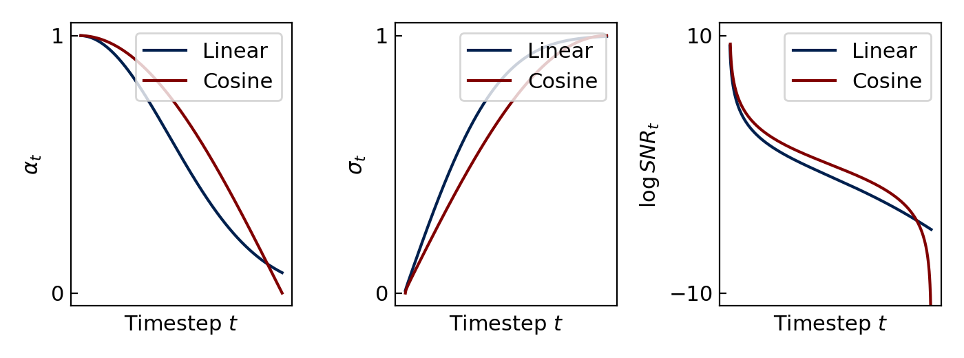
The figure conveys three linked observations.

First, the cosine schedule keeps the signal amplitude higher over much of the trajectory. In the left plot, the red cosine curve declines more slowly than the blue linear curve through the middle timesteps. Since signal power is ${\alpha }_t^2$, this indicates greater retained information at matched timestep indices.

Second, the cosine schedule adds noise more gradually through much of the process. In the center plot, its ${\sigma }_t$ rises later. This is the same fact viewed from the other side: when signal retention remains high, accumulated noise variance remains lower.

Third, the log-SNR plot shows why this matters for training and sampling. Over the main interior of the schedule, cosine maintains a higher log SNR than the linear schedule. A model trained at, say, $t=500$ therefore faces different denoising problems under the two schedules, even if both processes use $T=1000$ steps.

The final part of the cosine curve drops sharply. This is intentional: the forward process still needs to reach an approximately Gaussian terminal distribution. In a practical discrete implementation, clipping prevents the final ${\beta }_t$ from becoming exactly $1$.

There is no contradiction between these statements:

• Cosine ${\bar{\alpha }}_t$ changes gently near the beginning and end.
• Cosine log SNR changes very rapidly near idealized endpoints.

Near a clean sample, the noise variance approaches zero, so SNR tends toward infinity. Near pure noise, signal variance approaches zero, so SNR tends toward zero. Taking a logarithm makes both endpoint limits unbounded. The offset and variance clipping used in real schedules regularize those extremes.

---

A geometric view of the cosine schedule

Ignoring the small offset for a moment, a simple cosine construction is

$${\alpha }_t=\cos \left(\frac{\pi t}{2T}\right),{\sigma }_t=\sin \left(\frac{\pi t}{2T}\right).$$

It automatically satisfies

$${\alpha }_t^2+{\sigma }_t^2=1.$$

Let

$${\theta }_t=\frac{\pi t}{2T}.$$

Then $({\alpha }_t,{\sigma }_t)$ traces a quarter of the unit circle as ${\theta }_t$ moves from $0$ to $\pi /2$. Its SNR is

$${\mathrm{SNR}}_t=\frac{{\cos }^2{\theta }_t}{{\sin }^2{\theta }_t}={\cot }^2{\theta }_t.$$

At the equal-power point,

$${\alpha }_t^2={\sigma }_t^2=\frac{1}{2}.$$

For this idealized zero-offset schedule, that happens at

$${\theta }_t=\frac{\pi }{4},$$

which corresponds to the midpoint $t/T=1/2$.

This geometric picture is useful because it makes the schedule design tangible: a cosine schedule spaces the angle evenly, rather than increasing a local noise variance linearly. The practical offset version slightly modifies this ideal geometry, but preserves the same broad behavior.

---

Why the original linear schedule can waste late timesteps

With a standard linear ${\beta }_t$ schedule, the later per-step noise variances are the largest. Their effects compound after many earlier corruptions have already reduced ${\bar{\alpha }}_t$. Consequently, the process can reach extremely low SNR well before the nominal terminal time.

At very low SNR, a sample may be so close to isotropic Gaussian noise that additional forward steps change little that is relevant to image content. The improved-DDPM paper found that, for $32$ by $32$ and $64$ by $64$ images, this behavior made the end of the linear forward trajectory overly noisy. Their evidence included the observation that skipping a substantial late fraction of reverse steps did not materially worsen FID for a model trained with that schedule.

The key claim is not that every low-SNR timestep is useless. A generative model must learn to begin from noisy inputs. Rather, the concern is allocation: a fixed budget of $T$ discrete timesteps should cover meaningful changes in corruption level instead of repeatedly representing nearly indistinguishable noise-dominated states.

The cosine schedule reallocates that budget:

Schedule property	Linear ${\beta }_t$ schedule	Cosine ${\bar{\alpha }}_t$ schedule
Quantity designed directly	Per-step noise variance	Cumulative signal retention
Middle of trajectory	Signal may decay relatively quickly	Signal is retained longer
Late trajectory	Can spend many steps at very low SNR	Terminal loss of signal is concentrated later
Historical status	Original DDPM baseline	Common default in many later DDPM-style systems

“Common default” should not be read as a universal optimum. The best schedule depends on data resolution, model capacity, objective weighting, parameterization, and the sampler. But cosine scheduling is often a better baseline because it avoids an obvious mismatch between uniform timestep indexing and the information content of the noisy inputs.

---

Comparing schedules in code

The following code constructs both schedules in a form suitable for plotting. It recomputes the cosine cumulative product after clipping, so the displayed ${\bar{\alpha }}_t$ matches the actual discrete transition variances used by the model.

import math
import torch

T = 1000
eps = 1e-12

# Original DDPM-style linear beta schedule
betas_linear = torch.linspace(1e-4, 2e-2, T)
alpha_bar_linear = torch.cat(
    [
        torch.ones(1),
        torch.cumprod(1.0 - betas_linear, dim=0),
    ]
)

# Improved-DDPM cosine schedule
s = 0.008
t = torch.arange(T + 1, dtype=torch.float64) / T

f_t = torch.cos(((t + s) / (1.0 + s)) * math.pi / 2.0) ** 2
alpha_bar_target = f_t / f_t[0]

betas_cosine = 1.0 - alpha_bar_target[1:] / alpha_bar_target[:-1]
betas_cosine = betas_cosine.clamp(max=0.999)

alpha_bar_cosine = torch.cat(
    [
        torch.ones(1, dtype=torch.float64),
        torch.cumprod(1.0 - betas_cosine, dim=0),
    ]
)

def log_snr(alpha_bar):
    alpha_bar = alpha_bar.clamp(min=eps, max=1.0 - eps)
    return torch.log(alpha_bar) - torch.log1p(-alpha_bar)

log_snr_linear = log_snr(alpha_bar_linear)
log_snr_cosine = log_snr(alpha_bar_cosine)

When you plot log_snr_linear and log_snr_cosine against normalized time $t/T$, focus on three questions:

1. At which normalized times does each curve cross zero?
2. How much of the trajectory lies at strongly negative log SNR?
3. Does a fixed increment in timestep correspond to a comparably sized change in log SNR throughout the trajectory?

Those questions are more informative than asking only which schedule “adds noise faster.”

---

A disciplined interpretation

When comparing schedules, avoid four misleading shortcuts.

1. Do not equate timestep with noise level.
   Timestep $t=500$ is a label whose meaning depends entirely on the schedule.

2. Do not call the DDPM schedule linear in SNR.
   It is linear in ${\beta }_t$, while SNR depends nonlinearly on the product of all previous $1-{\beta }_s$.

3. Do not infer image recognizability solely from SNR.
   SNR gives an exact variance-based description of the corruption, but perceived structure also depends on the data distribution and image resolution.

4. Do not treat cosine as a magical functional form.
   The original authors explicitly describe the cosine squared choice as a convenient smooth shape. Its central contribution is a more sensible distribution of noise levels, not a uniquely privileged trigonometric formula.

---

Key takeaways

A linear DDPM schedule specifies linearly increasing per-step variances:

$${\beta }_t={\beta }_{\min }+\frac{t-1}{T-1}\left({\beta }_{\max }-{\beta }_{\min }\right).$$

Its cumulative signal retention,

$${\bar{\alpha }}_t=\prod _{s=1}^t(1-{\beta }_s),$$

and therefore its SNR profile are nonlinear.

The cosine schedule specifies cumulative signal retention more directly:

$${\bar{\alpha }}_t=\frac{{\cos }^2\left(\frac{t/T+s}{1+s}\frac{\pi }{2}\right)}{{\cos }^2\left(\frac{s}{1+s}\frac{\pi }{2}\right)}.$$

Compared at a common timestep index, cosine generally retains higher SNR through much of the trajectory, while bringing the sample to near-pure noise only near the end. This can prevent the late diffusion trajectory from being dominated by many nearly redundant, extremely low-SNR states.

Next, you will make these profiles concrete by implementing and visualizing forward diffusion on image data.