Signal-to-Noise Ratio Across Diffusion Timesteps

Hello. Previously, we collapsed the entire Gaussian forward chain into a direct conditional distribution:

$${\mathbf{x}}_t=\sqrt{{\bar{\alpha }}_t}{\mathbf{x}}_0+\sqrt{1-{\bar{\alpha }}_t}\mathbf{ϵ},\mathbf{ϵ}\sim \mathcal{N}(0,\mathbf{I}).$$

Here, ${\bar{\alpha }}_t$ is the cumulative product of the per-step retention factors. It tells us how much of the original sample remains at timestep $t$; $1-{\bar{\alpha }}_t$ is the variance of the accumulated Gaussian noise.

This lesson turns those two quantities into a single diagnostic: the signal-to-noise ratio, or SNR. You will learn to compute it from a diffusion schedule, interpret what high and low values mean, and use log SNR as a more convenient coordinate for reasoning about noise levels.

---

From the forward marginal to SNR

It helps to rename the two coefficients in the forward marginal:

$$a_t=\sqrt{{\bar{\alpha }}_t},{\sigma }_t=\sqrt{1-{\bar{\alpha }}_t}.$$

Then the forward process becomes

$${\mathbf{x}}_t=a_t{\mathbf{x}}_0+{\sigma }_t\mathbf{ϵ}.$$

The coefficient $a_t$ is the signal amplitude scale and ${\sigma }_t$ is the noise standard deviation. SNR, however, is defined in terms of power rather than amplitude. Since power or variance scales with the square of a coefficient,

$$\text{signal power}\propto a_t^2={\bar{\alpha }}_t,$$

and

$$\text{noise power}\propto {\sigma }_t^2=1-{\bar{\alpha }}_t.$$

Therefore, the conventional DDPM SNR at timestep $t$ is

$$\boxed{{\mathrm{SNR}}_t=\frac{{\bar{\alpha }}_t}{1-{\bar{\alpha }}_t}}$$

Equivalently, in the general notation ${\mathbf{x}}_t=\alpha (t){\mathbf{x}}_0+\sigma (t)\mathbf{ϵ}$,

$$\mathrm{SNR}(t)=\frac{\alpha (t{)}^2}{\sigma (t{)}^2}.$$

Be careful about notation across papers:

• In the previous lesson, ${\alpha }_t=1-{\beta }_t$ meant one-step retention.
• The total signal amplitude after $t$ steps is $\sqrt{{\bar{\alpha }}_t}$.
• Some continuous-time sources use $\alpha (t)$ for that total signal amplitude directly.

The underlying ratio is unchanged: square the total signal coefficient and divide by the total noise variance.

Strictly speaking, conditioned on a fixed ${\mathbf{x}}_0$, the signal component is deterministic rather than random. The “power” language becomes literal when data are approximately standardized so that each coordinate of ${\mathbf{x}}_0$ has unit variance. Under that convention,

$$\mathrm{Var}[{\mathbf{x}}_t]={\bar{\alpha }}_t+(1-{\bar{\alpha }}_t)=1.$$

This is why the common DDPM construction is called variance-preserving: as corruption grows, signal variance is exchanged for noise variance while the overall scale remains controlled.

---

Interpreting high, medium, and low SNR

SNR is a positive, dimensionless ratio. Its scale matters much more than its exact decimal representation.

SNR regime	Relation of powers	Meaning for ${\mathbf{x}}_t$	Denoising task
${\mathrm{SNR}}_t\gg 1$	Signal power dominates	The sample is close to ${\mathbf{x}}_0$	Remove a subtle perturbation
${\mathrm{SNR}}_t=1$	Signal and noise powers match	Both are equally present in variance terms	Recover substantial structure amid noise
${\mathrm{SNR}}_t\ll 1$	Noise power dominates	The input resembles Gaussian noise	Infer global, uncertain structure

At the beginning of the forward process,

$${\bar{\alpha }}_t\approx 1,$$

so

$${\mathrm{SNR}}_t=\frac{{\bar{\alpha }}_t}{1-{\bar{\alpha }}_t}$$

is very large. In the idealized clean limit where ${\bar{\alpha }}_0=1$, the denominator is zero and SNR is infinite: there is no added noise.

Late in the process,

$${\bar{\alpha }}_t\approx 0,$$

so

$${\mathrm{SNR}}_t\approx 0.$$

At this point, the noisy sample contains little direct evidence about the particular original image that produced it. The denoiser must rely increasingly on patterns learned from the data distribution.

A useful threshold is the equal-power point:

$${\mathrm{SNR}}_t=1.$$

Solving for ${\bar{\alpha }}_t$,

$$\frac{{\bar{\alpha }}_t}{1-{\bar{\alpha }}_t}=1,$$

gives

$${\bar{\alpha }}_t=\frac{1}{2}.$$

So signal and noise contribute equal variance exactly when half of the variance budget is attributed to retained data and half to added noise. This does not mean the image is necessarily half recognizable to a human; recognizability depends on image structure, resolution, and data normalization. But it is a reliable, model-independent statement about the forward process.

---

Computing SNR at a timestep

Suppose that at some timestep,

$${\bar{\alpha }}_t=\mathrm{0.8.}$$

Then

$$1-{\bar{\alpha }}_t=0.2,$$

and

$${\mathrm{SNR}}_t=\frac{0.8}{0.2}=4.$$

The retained signal has four times the power of the added noise.

Here are several representative values:

${\bar{\alpha }}_t$	Noise variance $1-{\bar{\alpha }}_t$	${\mathrm{SNR}}_t$	Interpretation
$0.99$	$0.01$	$99$	Very lightly corrupted
$0.90$	$0.10$	$9$	Signal clearly dominates
$0.50$	$0.50$	$1$	Equal signal and noise power
$0.10$	$0.90$	$0.111$	Noise dominates
$0.001$	$0.999$	approximately $0.001$	Almost pure noise

In an implementation, you generally start from a vector of ${\beta }_t$ values:

$${\alpha }_t=1-{\beta }_t,{\bar{\alpha }}_t=\prod _{s=1}^t{\alpha }_s.$$

You can then compute the full SNR curve with one elementwise division:

import torch

# betas has shape (T,); values must lie in (0, 1)
alphas = 1.0 - betas
alpha_bar = torch.cumprod(alphas, dim=0)

snr = alpha_bar / (1.0 - alpha_bar)

For a batch of random timesteps during training, gather the relevant cumulative values and reshape them for broadcasting over images:

B = x0.shape[0]
t = torch.randint(0, len(alpha_bar), (B,), device=x0.device)

ab = alpha_bar[t].view(B, 1, 1, 1)
snr_t = ab / (1.0 - ab)

In floating-point code, the earliest timesteps can have ${\bar{\alpha }}_t$ extremely close to $1$. If you will take logarithms or use SNR in a loss weight, guard against numerical infinities:

eps = 1e-8
ab_safe = ab.clamp(min=eps, max=1.0 - eps)

snr_t = ab_safe / (1.0 - ab_safe)
log_snr_t = torch.log(ab_safe) - torch.log1p(-ab_safe)

The clamp is a numerical precaution; it should not be interpreted as changing the mathematical endpoint of the diffusion process.

---

Why log SNR is often the better quantity

Raw SNR spans an enormous range. It may begin near infinity and end near zero, which makes a linear plot hard to read and an awkward scale for time-conditioning conventions.

Define the log SNR:

$${\lambda }_t=\log {\mathrm{SNR}}_t=\log {\bar{\alpha }}_t-\log (1-{\bar{\alpha }}_t).$$

Its interpretation is particularly clean:

• ${\lambda }_t>0$: signal power exceeds noise power.
• ${\lambda }_t=0$: equal signal and noise power.
• ${\lambda }_t<0$: noise power exceeds signal power.

Using a logarithm also turns multiplicative changes in SNR into additive changes in log SNR. For example, a change from SNR $100$ to $10$ is the same log-scale change as a move from $10$ to $1$, even though the raw differences are very different.

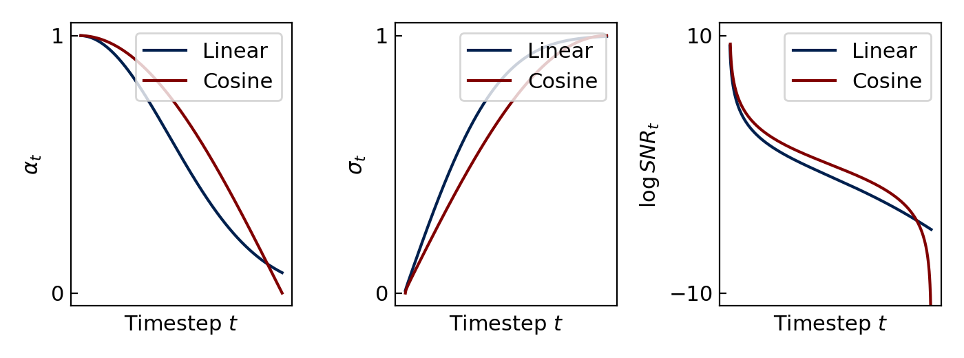
The schedule figure has an important message: a timestep is not intrinsically meaningful. Two schedules can use the same number of timesteps and both end at near-pure noise, while assigning very different SNR values to their intermediate steps. Therefore, the reverse model is really learning a family of denoising problems indexed by noise level.

The short excerpt below gives a visual motivation for this distinction before the next lesson examines the linear and cosine profiles more carefully.

---

A final distinction: noise level versus timestep

It is tempting to say “early timestep” and “low noise” interchangeably. That is only safe after specifying a schedule. The robust description is based on ${\bar{\alpha }}_t$, SNR, or log SNR:

$${\bar{\alpha }}_t⟺{\mathrm{SNR}}_t⟺{\lambda }_t.$$

For the standard variance-preserving process, each of these determines the others:

$${\bar{\alpha }}_t=\frac{{\mathrm{SNR}}_t}{1+{\mathrm{SNR}}_t},$$

and

$${\mathrm{SNR}}_t=\exp ({\lambda }_t).$$

This equivalence will become useful later when discussing model parameterizations and loss weighting. For now, the practical principle is simple: whenever you want to know how difficult a denoising timestep is, inspect its SNR rather than relying on its index alone.

---

Key takeaways

For DDPM forward diffusion,

$${\mathbf{x}}_t=\sqrt{{\bar{\alpha }}_t}{\mathbf{x}}_0+\sqrt{1-{\bar{\alpha }}_t}\mathbf{ϵ},$$

the signal and noise powers are respectively ${\bar{\alpha }}_t$ and $1-{\bar{\alpha }}_t$. Thus,

$$\boxed{{\mathrm{SNR}}_t=\frac{{\bar{\alpha }}_t}{1-{\bar{\alpha }}_t}}$$

is the central measure of corruption level.

High SNR means the input is mostly retained signal; low SNR means it is dominated by random noise. The equal-power point occurs at ${\bar{\alpha }}_t=0.5$, where ${\mathrm{SNR}}_t=1$. Log SNR provides a stable and comparable scale:

$$\log {\mathrm{SNR}}_t=\log {\bar{\alpha }}_t-\log (1-{\bar{\alpha }}_t).$$

Next, we will compare linear and cosine noise schedules by studying how each one distributes SNR across the diffusion trajectory.