Calculating Gradients of Multivariable Functions

Hello! Welcome back to our course on the mathematical foundations of AI.

Introduction

In our previous lesson, we established how to compute partial derivatives, which measure the rate of change of a multivariable function along the directions of the coordinate axes. This was like finding the slope of a hill, but only when walking strictly east or strictly north.

This is a good start, but in machine learning, we're often interested in a more powerful question: from our current position, what is the single best direction to move in to achieve the fastest increase (or decrease) in our function's value? Answering this is the key to optimizing complex models.

Today, we will address this by learning to compute the gradient of a scalar-valued multivariable function. We will see that the gradient is a vector that elegantly packages all the partial derivatives of a function into a single object. This vector not only tells us the rate of change in all axial directions at once but, more importantly, points in the direction of the steepest ascent of the function.

Defining the Gradient

The concept of the gradient builds directly on what we learned about partial derivatives. For a scalar-valued function of $n$ variables, $f(x_1,x_2,\dots ,x_n)$, the gradient is simply the vector whose components are the partial derivatives of $f$ with respect to each variable.

Given your linear algebra background from Module 1, you'll recognize this as a column vector. The gradient of $f$ is denoted by $\nabla f$ (pronounced "nabla f" or "del f").

Formal Definition:
Let $f:{\mathbb{R}}^n\to \mathbb{R}$ be a differentiable scalar-valued function with variables $\mathbf{x}=(x_1,x_2,\dots ,x_n)$. The gradient of $f$ is the vector-valued function:

$$\nabla f(\mathbf{x})=\left[\begin{array}{c}\frac{\partial f}{\partial x_1}\\ \frac{\partial f}{\partial x_2}\\ ⋮\\ \frac{\partial f}{\partial x_n}\end{array}\right]$$

Note that the gradient takes a point in ${\mathbb{R}}^n$ (like a specific set of model parameters) and returns a vector in ${\mathbb{R}}^n$ (the direction of steepest ascent at that point).

For a function of two variables, $f(x,y)$, the gradient is:
$\nabla f(x,y)=⟨\frac{\partial f}{\partial x},\frac{\partial f}{\partial y}⟩=\left[\begin{array}{c}{f}_x(x,y)\\ f_y(x,y)\end{array}\right]$

Computing the Gradient

The process of computing the gradient is straightforward:

1. Identify all the independent variables of the function.
2. Compute the partial derivative of the function with respect to each variable, as you learned in the previous lesson.
3. Arrange these partial derivatives into a vector.

Let's watch a video that illustrates this computational process.

As the video showed, for $f(x_1,x_2)=x_1^2+x_2^2$:

• $\frac{\partial f}{\partial x_1}=2x_1$
• $\frac{\partial f}{\partial x_2}=2x_2$

So, the gradient is:
$\nabla f(x_1,x_2)=\left[\begin{array}{c}2x_1\\ 2x_2\end{array}\right]=2\left[\begin{array}{c}{x}_1\\ x_2\end{array}\right]=2\mathbf{x}$

At a specific point, say $(3,4)$, the gradient vector would be $\nabla f(3,4)=\left[\begin{array}{c}6\\ 8\end{array}\right]$.

Test your understanding!

Let $f(x,y,z)=x^{2}y+z\sin (x)$. Compute the gradient of $f$, $\nabla f(x,y,z)$.

Show answer

First, we compute the three partial derivatives:

1. $\frac{\partial f}{\partial x}=\frac{\partial }{\partial x}(x^{2}y+z\sin (x))=2xy+z\cos (x)$
2. $\frac{\partial f}{\partial y}=\frac{\partial }{\partial y}(x^{2}y+z\sin (x))=x^2$
3. $\frac{\partial f}{\partial z}=\frac{\partial }{\partial z}(x^{2}y+z\sin (x))=\sin (x)$

Now, we assemble them into the gradient vector:
$\nabla f(x,y,z)=\left[\begin{array}{c}2xy+z\cos (x)\\ x^2\\ \sin (x)\end{array}\right]$

The Geometric Meaning of the Gradient

Computing the gradient is just mechanics. The reason it's a cornerstone of machine learning lies in its geometric interpretation. To understand this, we first need to introduce the concept of a directional derivative.

The partial derivatives $\frac{\partial f}{\partial x}$ and $\frac{\partial f}{\partial y}$ tell us the rate of change in the directions of the unit vectors $\mathbf{i}=⟨1,0⟩$ and $\mathbf{j}=⟨0,1⟩$. The directional derivative, $D_{\mathbf{u}}f$, generalizes this to find the rate of change in the direction of any unit vector $\mathbf{u}$.

A remarkable result from calculus is that the directional derivative can be computed elegantly using the gradient. For a differentiable function $f$ and a unit vector $\mathbf{u}$, the directional derivative of $f$ in the direction of $\mathbf{u}$ is given by the dot product of the gradient and $\mathbf{u}$:

$D_{\mathbf{u}}f=\nabla f\cdot \mathbf{u}$

This single equation is packed with meaning. To fully appreciate its derivation and implications, we'll consult a rigorous textual explanation.

Now, let's unpack the implications of the formula $D_{\mathbf{u}}f=\nabla f\cdot \mathbf{u}$. Recall from linear algebra that the dot product can also be written as $\mathbf{a}\cdot \mathbf{b}=\Vert \mathbf{a}\Vert \Vert \mathbf{b}\Vert \cos (\theta )$, where $\theta$ is the angle between the vectors $\mathbf{a}$ and $\mathbf{b}$.

Applying this to the directional derivative:
$D_{\mathbf{u}}f=\Vert \nabla f\Vert \Vert \mathbf{u}\Vert \cos (\theta )=\Vert \nabla f\Vert \cos (\theta )$
(since $\Vert \mathbf{u}\Vert =1$).

This tells us everything we need to know:

• Maximum Increase: The rate of change $D_{\mathbf{u}}f$ is maximized when $\cos (\theta )=1$, which happens when $\theta =0$. This means the direction $\mathbf{u}$ points in the same direction as the gradient $\nabla f$. The value of this maximum rate of change is $\Vert \nabla f\Vert$.
• Maximum Decrease: The rate of change is minimized (most negative) when $\cos (\theta )=-1$, which happens when $\theta =\pi$. This means $\mathbf{u}$ points in the opposite direction of the gradient, $-\nabla f$. The value of this maximum rate of decrease is $-\Vert \nabla f\Vert$.
• Zero Change: The rate of change is zero when $\cos (\theta )=0$, which happens when $\theta =\pi /2$. This means $\mathbf{u}$ is orthogonal (perpendicular) to the gradient $\nabla f$. This direction is tangent to the level curve of the function at that point.

In summary:

The gradient vector $\nabla f$ at a point $\mathbf{p}$ points in the direction of the steepest ascent of the function $f$ at $\mathbf{p}$, and its magnitude $\Vert \nabla f(\mathbf{p})\Vert$ is the rate of that ascent.

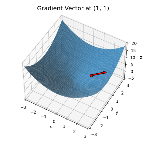
Connection to Machine Learning: Gradient Descent

This brings us to the core application in machine learning. Most ML training involves minimizing a cost function (or loss function), often denoted $J(\theta )$, where $\theta$ is the vector of model parameters. We want to find the parameters $\theta$ that make the cost as low as possible.

The gradient, $\nabla J(\theta )$, tells us the direction to change $\theta$ to increase the cost the fastest. Therefore, the negative gradient, $-\nabla J(\theta )$, points in the direction of the steepest decrease in cost.

The gradient descent algorithm is built on this exact principle:

1. Start with some random initial parameters $\theta$.
2. Calculate the negative gradient of the cost function, $-\nabla J(\theta )$.
3. Update the parameters by taking a small step in that direction: ${\theta }_{\text{new}}={\theta }_{\text{old}}-\alpha \nabla J(\theta )$, where $\alpha$ is a small positive number called the learning rate.
4. Repeat steps 2 and 3 until the cost converges to a minimum.

Every time you train a neural network using libraries like PyTorch or TensorFlow, this is fundamentally what's happening under the hood during the optimization step.

Conclusion

In this lesson, we have defined the gradient and established its critical role in multivariate calculus and machine learning.

Key Takeaways:

• The gradient, $\nabla f$, is a vector containing all the partial derivatives of a scalar-valued function $f$.
• To compute the gradient, you calculate each partial derivative individually and assemble them into a vector.
• The directional derivative $D_{\mathbf{u}}f=\nabla f\cdot \mathbf{u}$ gives the rate of change of $f$ in any direction $\mathbf{u}$.
• The gradient's direction is the direction of the function's steepest ascent, and its magnitude is the rate of that ascent.
• The negative gradient, $-\nabla f$, points in the direction of steepest descent, forming the basis for the gradient descent optimization algorithm.

Preview of the Next Lesson:
So far, we've dealt with relatively simple functions. In machine learning, especially in deep learning, functions are often complex compositions of other functions (e.g., an activation function applied to a linear transformation). To find the gradient of such a composite function, we need a multivariable version of a familiar tool: the chain rule. In the next lesson, we will derive the multivariable chain rule and see how it allows us to compute gradients for these more complex, nested functions.