Chain Rule for Multiple Variables

Recommended resources

The freely available resources this lesson will direct you to.

Hello! Welcome to your next lesson on the mathematical foundations of AI.

Introduction

In our last lesson, we defined the gradient, $\nabla f$ , and established its geometric meaning as the direction of a function's steepest ascent. This is a crucial tool for optimization. However, the functions we optimize in machine learning, such as the cost function of a neural network, are rarely simple. They are almost always composite functions, where the output of one function becomes the input to another.

For example, a single neuron might compute a linear combination of its inputs, $z = w \cdot x + b$ , and then pass this result through a non-linear activation function, $a = σ (z)$ . To optimize the weights $w$ using gradient descent, we need to find the gradient of the final loss with respect to $w$ , which requires us to 'look through' the composition of functions.

Today, we will learn how to do this by deriving and applying the chain rule for composite functions in multiple variables. This powerful rule is the fundamental mechanism behind the backpropagation algorithm, which is used to train virtually all modern neural networks. You will see how the component-wise intuition from single-variable calculus extends to a far more elegant and powerful formulation using the linear algebra you've already mastered.

The Chain Rule: From Components to Matrices

Let's start with an intuitive picture. Imagine a function $z = f (x, y)$ , where the intermediate variables $x$ and $y$ are themselves functions of other variables, say $s$ and $t$ . So, $x = g (s, t)$ and $y = h (s, t)$ . The final output $z$ is therefore a composite function of $s$ and $t$ .

How does a small change in $s$ affect the final output $z$ ? The change propagates along all possible paths in the dependency graph.

Multivariable Chain Rule Illustration — This diagram illustrates the dependency structure. A change in 's' influences both 'x' and 'y', and these changes in turn influence 'f'. The chain rule sums the effects of these two paths.

This dependency suggests that the total change in $z$ with respect to $s$ is the sum of the changes propagated through $x$ and $y$ . This gives us the component-wise form of the chain rule:

\frac{\partial z}{\partial s} = \frac{\partial z}{\partial x} \frac{\partial x}{\partial s} + \frac{\partial z}{\partial y} \frac{\partial y}{\partial s}

And similarly for $t$ :

\frac{\partial z}{\partial t} = \frac{\partial z}{\partial x} \frac{\partial x}{\partial t} + \frac{\partial z}{\partial y} \frac{\partial y}{\partial t}

This form is useful, but it can become incredibly cumbersome with more variables and deeper compositions. Your background in data structures and algorithms might lead you to appreciate that we need a more scalable and systematic representation. This is where linear algebra comes in.

The Derivative as a Linear Map

To generalize the chain rule elegantly, we must first upgrade our view of the derivative. For multivariable functions, the derivative at a point is not just a number (a slope) but the best linear approximation of the function's change near that point. This linear approximation is a linear map, which can be represented by a matrix.

This matrix of all first-order partial derivatives has a special name: the Jacobian matrix.

A note on the multivariable chain rule

To formalize the chain rule, we first need to reinterpret the derivative. This note from the Stanford AI Lab explains the concept of the derivative as a linear map and defines the Jacobian matrix, which is the matrix representation of this map.

Please read the sections 'The derivative as a linear map' and 'Jacobian and gradient'. Pay close attention to how the total derivative is defined as a linear map and how the Jacobian matrix emerges as its numerical implementation. Note the connection between the gradient (which we know) and the Jacobian of a scalar-valued function.

As the reading explains:

For a vector-valued function $g : R^{n} \to R^{m}$ , its derivative is the Jacobian matrix $J_{g}$ , an $m \times n$ matrix of partial derivatives.
For a scalar-valued function $f : R^{n} \to R$ , its Jacobian is a $1 \times n$ row vector. This is simply the transpose of the gradient vector we studied in the last lesson: $J_{f} = (\nabla f)^{T}$ .

The Chain Rule as Matrix Multiplication: The Formal Proof

With this new perspective, the chain rule becomes a beautifully simple statement: the derivative of a composition of functions is the composition of their derivatives. Since the derivatives are linear maps (matrices), their composition is simply matrix multiplication.

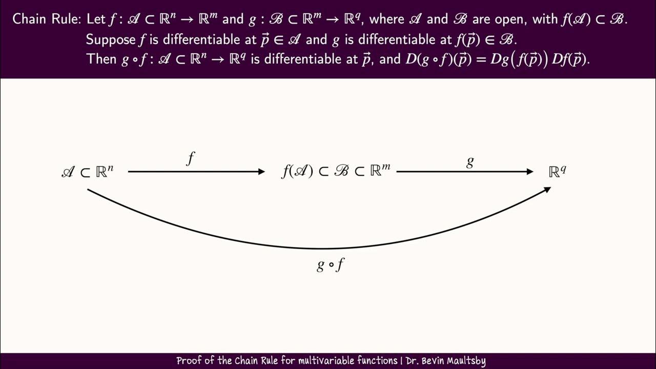
Multivariable Chain Rule Definition and Diagram — This image states the main theorem. For a composite function (g ∘ f), its derivative matrix is the product of the derivative matrices of g and f, evaluated at the correct points.

Now, let's go through the formal derivation. Your preference for mathematical rigor will be satisfied here. The following document proves this theorem concisely by composing the linear approximations of the functions.

The Multivariable Chain Rule

Now, let's walk through a concise and formal derivation of the chain rule. This document from UC Berkeley uses the idea of linear approximation and o() notation to show how composing functions leads directly to multiplying their derivative matrices (Jacobians).

Read the entire short document. Section 1 formalizes the linear approximation for multivariable functions. Pay close attention to how f and g are approximated by matrices Df and Dg (which are Jacobians). The key result is on page 2, where composing the approximations leads to the matrix product Df◦g = DfDg. The conceptual summary at the end ties it all together.

Let's connect this back to our initial example: $z = f (x, y)$ where $(x, y) = g (s, t)$ .

The function $f : R^{2} \to R$ is scalar-valued. Its derivative matrix $D_{f}$ is its Jacobian, a $1 \times 2$ matrix:
$D_{f} = J_{f} = (\nabla f)^{T} = [\frac{\partial f}{\partial x} \frac{\partial f}{\partial y}]$
The function $g : R^{2} \to R^{2}$ is vector-valued. Its derivative matrix $D_{g}$ is its Jacobian, a $2 \times 2$ matrix:
$D_{g} = J_{g} = [\frac{\partial x}{\partial s} \frac{\partial y}{\partial s} \frac{\partial x}{\partial t} \frac{\partial y}{\partial t}]$

The chain rule states that the derivative of the composite function, $D_{f \circ g}$ , is the product of these matrices:

D_{f \circ g} = D_{f} D_{g} = [\frac{\partial f}{\partial x} \frac{\partial f}{\partial y}] [\frac{\partial x}{\partial s} \frac{\partial y}{\partial s} \frac{\partial x}{\partial t} \frac{\partial y}{\partial t}]

Performing the matrix multiplication gives:

D_{f \circ g} = [(\frac{\partial f}{\partial x} \frac{\partial x}{\partial s} + \frac{\partial f}{\partial y} \frac{\partial y}{\partial s}) (\frac{\partial f}{\partial x} \frac{\partial x}{\partial t} + \frac{\partial f}{\partial y} \frac{\partial y}{\partial t})]

The resulting $1 \times 2$ matrix contains the partial derivatives of the composite function with respect to $s$ and $t$ . You can see that this single matrix equation elegantly reproduces the two component-wise formulas we started with.

Test your understanding!

Let's consider a slightly more complex composition relevant to neural networks. Let $L$ be a scalar loss, which is a function of a vector $a \in R^{m}$ . The vector $a$ is a function of a vector $z \in R^{n}$ , so $a = g (z)$ . The vector $z$ is a linear function of an input vector $x \in R^{d}$ , given by $z = W x$ , where $W$ is an $n \times d$ weight matrix. The full composition is $L (x) = f (g (W x))$ .

Our goal is to find the derivative of the loss $L$ with respect to the input $x$ , which is the Jacobian $D_{L} (x)$ . Use the chain rule in matrix form to write down an expression for $D_{L} (x)$ in terms of the Jacobians of $f$ , $g$ , and the linear transformation.

Show answer

Let $h (x) = W x$ . Then the composition is $L = f (g (h (x)))$ .
Applying the chain rule repeatedly:
$D_{L} (x) = D_{f} (g (h (x))) \cdot D_{g} (h (x)) \cdot D_{h} (x)$

Let's look at the dimensions:

$D_{f}$ is the Jacobian of $f : R^{m} \to R$ , so it is a $1 \times m$ matrix (a row vector).
$D_{g}$ is the Jacobian of $g : R^{n} \to R^{m}$ , so it is an $m \times n$ matrix.
The function $h (x) = W x$ is a linear transformation. Its derivative with respect to $x$ is simply the matrix $W$ itself, which is $n \times d$ .

So, the final product is:
$D_{L} (x) = (1 \times m matrix) \cdot (m \times n matrix) \cdot (n \times d matrix)$
The result is a $1 \times d$ matrix, which is exactly the correct shape for the Jacobian of the scalar-valued function $L (x)$ with respect to the $d$ -dimensional input $x$ . This systematic, dimension-aware process is the essence of backpropagation.

Conclusion

Today, we have formally derived the multivariable chain rule, a pivotal concept for your goal of understanding the theory behind modern AI.

Key Takeaways:

The derivative of a multivariable function can be seen as its best linear approximation, represented by the Jacobian matrix.
The chain rule for composite functions $(g \circ f)$ elegantly simplifies to the multiplication of their Jacobian matrices: $J_{g \circ f} = (J_{g} \circ f) \cdot J_{f}$ .
This matrix formulation is not only more general and powerful than the component-wise approach but is also the fundamental principle that enables the computation of gradients in complex, deeply nested functions like neural networks (i.e., backpropagation).
The gradient $\nabla f$ is a special case of the Jacobian for scalar-valued functions, where $J_{f} = (\nabla f)^{T}$ .

Preview of the Next Lesson:
We've now formally introduced the Jacobian matrix and seen its role in the chain rule. In the next lesson, we will focus exclusively on the Jacobian. We will solidify our understanding by learning how to compute the Jacobian matrix for a vector-valued function and interpret its meaning, preparing us for more advanced topics in optimization and model analysis.