Analyzing Time and Auxiliary-Space Complexity in Python Collections

Hello! Last lesson, you used dictionaries to count values and sets to record what you had seen. Those choices also affect how a solution performs: checking membership in a list can cost more than checking it in a set, while a set consumes extra memory.

This lesson gives you a way to determine time complexity and auxiliary-space complexity from short Python functions. You’ll use it to explain the cost of familiar counting and duplicate-detection patterns, rather than guessing from the number of lines of code.

Measure growth, not seconds

Let $n$ be the number of items in an input list. Time complexity describes how the amount of work grows as $n$ grows; it does not predict an exact running time in seconds. A function that visits every item once generally takes $O(n)$ time. One that checks every item against every other item may take $O(n^2)$.

Watch Greg Hogg’s Time & Space Complexity – Big O Notation for the contrast between a single pass and processing pairs, then for the rules used to simplify a complexity expression.

Big O expresses an asymptotic upper bound: a bound on growth for sufficiently large inputs. In coding-problem discussions, we usually give the tightest useful Big O bound for the case being analyzed, often the worst-case input.

For example, two separate passes over a list perform roughly $2n$ visits. We report $O(n)$, because doubling $n$ still roughly doubles the work. If a function performs a quadratic task plus one pass, we report $O(n^2)$: the quadratic term dominates as $n$ grows.

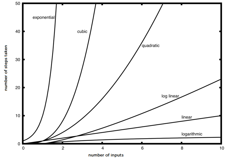
A useful starting question is therefore: What changes when the input gets one item larger? Does the function do one more small piece of work, or does it search an increasingly large collection again?

Assign a cost to each Python operation

A loop count alone is not enough. You also need to know what happens inside the loop. Python’s in operator, for instance, looks identical in x in values and x in seen, but its cost depends on whether values is a list and seen is a set.

Tech With Tim’s Python Sets Tutorial #1 & Time Complexity (BIG O) demonstrates this membership contrast.

Keep the Python Wiki’s TimeComplexity reference nearby when analyzing code. You do not need to memorize every row: concentrate on the operations used in short list-, set-, and dictionary-based solutions.

Here are the costs most relevant today:

A list membership test may inspect every item before returning False. Insertion near the front shifts existing elements. Appending usually avoids that shifting; amortized $O(1)$ means occasional costly resizes are spread across many appends.

Sets and dictionaries use hashing for their typical fast lookups. Their $O(1)$ entries are not guarantees for every individual operation: collisions or resizing can make an operation slower. Standard DSA analysis usually assumes hashable, reasonably bounded-size values and reports the average or expected hash-table cost. For a list search, by contrast, the $O(n)$ worst case is easy to encounter—search for something absent.

Read the whole function, including hidden work

Consider the frequency counter from the previous lesson:

def frequencies(items):
    counts = {}
    for x in items:
        counts[x] = counts.get(x, 0) + 1
    return counts

If there are $n$ items, the loop runs $n$ times. Each dictionary lookup and assignment takes $O(1)$ average time under the usual hashing assumptions. Thus the total is $O(n)$ average time, even if some values repeat.

Now compare two ways to detect a duplicate:

def has_repeat_list(items):
    seen = []
    for x in items:
        if x in seen:
            return True
        seen.append(x)
    return False


def has_repeat_set(items):
    seen = set()
    for x in items:
        if x in seen:
            return True
        seen.add(x)
    return False

Both loops can visit $n$ items. But when all items are distinct, has_repeat_list searches a growing list on each visit. The searches examine up to zero items, then one, then two, and so on. Their combined work grows as $O(n^2)$. In has_repeat_set, each membership check and addition is $O(1)$ on average, so the whole function takes $O(n)$ average time.

Notice the role of return True: a duplicate near the start can make either function finish quickly. The complexities above describe the worst-case input for the list version and the usual hash-table-cost analysis for the set version, not the time of every call.

The same caution applies to compact Python syntax. A slice such as items[:] copies $n$ references and takes $O(n)$ time; it is not free because it occupies one line. When analyzing a short solution, expand each substantial operation into its cost before combining costs.

If a function has two inputs of different sizes, name both. For example, a list of $n$ stored values and $m$ queries can require $O(nm)$ time if every query searches the list. Building a set once and then checking all queries typically costs $O(n+m)$ time. Replacing both sizes with a single $n$ would hide that distinction.

Count extra memory separately

Auxiliary space is memory the algorithm uses in addition to its given input. A loop variable or a running count uses $O(1)$ extra space. A newly built collection can grow with the input.

Watch the space comparison in Greg Hogg’s video before revisiting the functions above.

Let $u$ be the number of distinct values among $n$ input items. In frequencies, the dictionary holds $u$ entries, so auxiliary space is $O(u)$, which is at most $O(n)$. Both duplicate detectors also retain up to $u$ seen values: each uses $O(u)$ auxiliary space in the worst case, although their time costs differ.

This distinction prevents a common mistake: a function does not have $O(1)$ auxiliary space merely because it returns one Boolean or one number. Its temporary set or dictionary still occupies memory while it runs. Conversely, repeatedly searching a list can be slow even when a function stores only a few variables.

For another familiar expression:

def distinct_count(items):
    return len(set(items))

Building set(items) visits the $n$ input values, so it takes $O(n)$ average time. The temporary set holds $u$ values, giving $O(u)$ auxiliary space. The final result is only one integer, but the temporary set counts.

When writing an analysis, state whether you are counting a newly constructed output collection as extra space. For this lesson, count all new collections a function allocates, including one it returns; exclude only the input supplied to it. That convention makes analyses of short Python functions consistent.

A reliable reading order for code is:

1. Define input sizes, such as $n$, $m$, and—when duplicates matter—$u$.
2. Count how often each block executes, including early exits and nested loops.
3. Charge for operations inside those blocks, especially searches, copies, and hash-table operations.
4. Combine the time costs, keeping the dominant growth term.
5. Separately count the largest amount of additional storage held at one time.

Key takeaways

A loop over $n$ items is not automatically $O(n)$: its body may perform a list search that also grows with $n$. List membership takes $O(n)$ in the worst case, while set and dictionary membership are $O(1)$ on average under standard hashing assumptions. For auxiliary space, count the new lists, sets, and dictionaries a function holds—not just the size of its final answer.

In the next lesson, you’ll use a running state to solve a one-pass array or string problem. You’ll be able to judge both what that state must remember and what it costs.