KCL for Node Voltages

Hello! Welcome back.

In our last lesson, we established the foundation for nodal analysis by learning how to identify nodes, choose a reference, and assign unknown potential variables (v_1, v_2, etc.). We concluded that this set of N-1 node potentials is sufficient to describe the entire state of a circuit.

Today, we build directly on that foundation. Our goal is to translate the physical principle of Kirchhoff's Current Law into a set of solvable mathematical equations. Your learning outcome is to: Formulate KCL equations at each non-reference node in terms of unknown node voltages.

This is the crucial step where the circuit diagram becomes a system of algebraic equations. Mastering this procedure transforms circuit analysis from an ad-hoc process into a systematic, almost algorithmic one—a logical framework that I believe you'll find quite powerful.

1. The Core Principle: KCL in Terms of Node Voltages

From a previous lesson, we know that Kirchhoff's Current Law (KCL) is a statement of the conservation of charge: the total current entering any node must equal the total current leaving it. A common way to state this is:

The algebraic sum of currents leaving a node is zero.

This is the principle we will apply. The key to nodal analysis is how we express these currents. Instead of using variables like i_1 or i_2, we will write each current directly in terms of the node potentials and resistances using Ohm's Law.

For a resistor R connected between two nodes, say node A (at potential v_A) and node B (at potential v_B), the current flowing from A to B is:
$i_{A\to B}=\frac{\text{Potential at starting node}-\text{Potential at ending node}}{\text{Resistance}}=\frac{v_A-v_B}{R}$
This single expression is the engine of nodal analysis.

2. A Systematic Procedure for Writing Nodal Equations

To avoid confusion with signs, we will adopt a consistent convention: For any node we are analyzing, we will assume all unknown currents are flowing out of that node.

This leads to a clear, repeatable process:

1. Identify and label: Identify all nodes, choose a reference node (ground = 0V), and label the potentials of all other nodes (v_1, v_2, ...). This was covered in our last lesson.
2. Select a node: Pick one of the non-reference nodes to analyze.
3. Write the KCL equation: Write one KCL equation for this node by summing the currents leaving it and setting the sum to zero.
   • For each resistor connected to the node, the current leaving is (V_your_node - V_other_side) / R.
   • For a current source, if it directs current away from your node, it's a positive term in the sum. If it directs current into your node, it's a negative term.
4. Repeat: Repeat steps 2 and 3 for every other non-reference node.

You will end up with N-1 equations for your N-1 unknown node potentials.

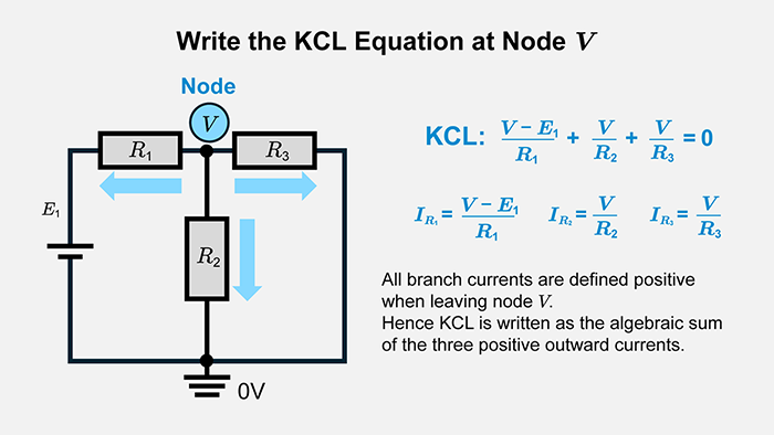
This image provides a perfect illustration of this principle for a single node V.

3. Guided Example: A Circuit with One Unknown Node

Let's apply this method to a circuit that yields a single equation. The goal here is to focus purely on the formulation step.

Let's walk through that same process with our systematic convention. Consider the circuit from the video.

A circuit with two voltage sources and one unknown node potential, v_a.

1. Nodes: We have three nodes. The bottom is the reference (0V). The nodes on the left and right are connected to voltage sources, so their potentials are known: 3V and 2V, respectively. There is only one unknown node potential, v_a.
2. Select Node: We select node a for analysis.
3. Write KCL: We will sum the currents leaving node a.
   • Current leaving through the 2Ω resistor: (v_a - 3V) / 2Ω
   • Current leaving through the 4Ω resistor: (v_a - 2V) / 4Ω
   • Current leaving through the 1Ω resistor: (v_a - 0V) / 1Ω

The KCL equation is the sum of these currents set to zero:
$\frac{v_a-3}{2}+\frac{v_a-2}{4}+\frac{v_a-0}{1}=0$

This is the formulated equation for the node. Notice that if you assume currents are leaving the node, the node's own voltage (v_a) will always appear as the positive term in each numerator. This is a great way to check your work.

4. Guided Example: A Circuit with Multiple Unknown Nodes

When a circuit has more than one unknown node potential, the process is the same, but you repeat it for each node, generating a system of simultaneous equations.

Let's look at a typical two-node problem.

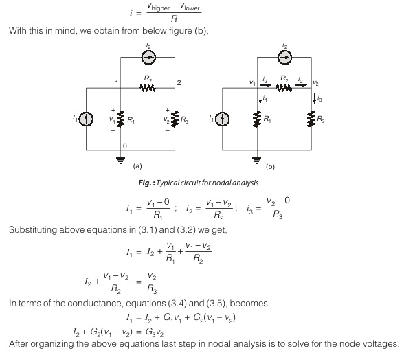
Let's formulate the equations for the circuit in the image above, following our systematic procedure.

Node 1 (at potential v_1):
Sum the currents leaving node 1 and set to zero.

• The source I_1 is entering, so it contributes -I_1 to the sum of leaving currents.
• Current leaving through R_1: (v_1 - 0) / R_1
• Current leaving through R_3: (v_1 - v_2) / R_3

Equation for node 1:
$-I_1+\frac{v_1}{R_1}+\frac{v_1-v_2}{R_3}=0$

Node 2 (at potential v_2):
Sum the currents leaving node 2 and set to zero.

• The source I_2 is leaving, so it contributes +I_2.
• Current leaving through R_3 (flowing from v_2 to v_1): (v_2 - v_1) / R_3
• Current leaving through R_2: (v_2 - 0) / R_2

Equation for node 2:
$I_2+\frac{v_2-v_1}{R_3}+\frac{v_2}{R_2}=0$
We now have two equations and two unknowns (v_1, v_2). The problem has been successfully translated into a system of linear equations.

Your Turn: Practice Formulation

Now it's your turn to apply the procedure. For the circuit below, your task is to write the KCL equations for the non-reference nodes (v_1 and v_2). Do not solve them yet.

A practice circuit with one voltage source, one current source, and two unknown node potentials.

1. Identify the non-reference nodes (they are already labeled v_1 and v_2). The bottom node is the ground reference (0V).
2. Write the KCL equation for node v_1.
3. Write the KCL equation for node v_2.

Conclusion

Today we've mastered the core procedure of nodal analysis: converting a circuit schematic into a system of equations. This is a major step towards being able to solve any resistive DC circuit, no matter how complex its topology.

Key Takeaways:

• Nodal analysis is the application of KCL at each non-reference node.
• The key is to express each branch current using Ohm's Law in terms of the node potentials: I = (V_start - V_end) / R.
• Adopting a consistent convention, such as "sum of currents leaving the node is zero," makes the process systematic and less prone to errors.
• The result is a system of N-1 linear equations for the N-1 unknown node potentials.

Preview of the Next Lesson:
We have successfully set up the problem. The next logical step is to solve it. In the next lesson, we will focus on the algebraic techniques—from simple substitution to more formal methods—to solve the system of linear equations and find the actual numerical values for the node voltages and branch currents. Your strong algebra background will be a great asset here.