Beyond L2: Exploring L1 and Early Stopping for Regularization

Introduction

In our previous lessons, we've developed a comprehensive toolkit for training neural networks. We've explored advanced optimizers, weight initialization strategies, and methods like Dropout and Batch Normalization. We also derived L2 regularization (weight decay), a technique that penalizes the squared magnitude of the weights to prevent overfitting. This method encourages the model to use smaller, more distributed weights.

In this lesson, we will expand our understanding of regularization by examining two other classical yet powerful techniques. As per the learning outcome, this will be a conceptual overview designed to supplement your core knowledge, providing crucial context for both classical machine learning and modern deep learning practices. We will explore L1 regularization and its remarkable ability to induce sparsity, and early stopping, a fundamentally different, procedural approach to preventing overfitting. These methods offer alternative philosophies for controlling model complexity, each with unique mathematical underpinnings and practical implications.

L1 Regularization: Engineering Sparsity

Recall that L2 regularization adds a penalty proportional to the sum of the squared weights ($||\mathbf{w}|{|}_2^2$) to the loss function. This pulls weights toward zero but rarely makes them exactly zero.

Now, consider a scenario where you are working with a model that has thousands or even millions of features (e.g., in natural language processing or genomics). You might hypothesize that many of these features are irrelevant to the task. How might you design a regularizer that not only prevents overfitting but also performs automatic feature selection by forcing the weights of irrelevant features to become precisely zero?

This is the core idea behind L1 regularization, also known as Lasso (Least Absolute Shrinkage and Selection Operator) in the context of linear models. The L1 penalty is proportional to the sum of the absolute values of the weights, defined by the L1 norm:

$$||\mathbf{w}|{|}_1=\sum _i|w_i|$$

The regularized loss function then becomes:

$$J_{\text{L1}}(\mathbf{w})=J_{\text{original}}(\mathbf{w})+\lambda \sum _i|w_i|$$

The key effect of this change is that L1 regularization produces sparse models, where many weights are exactly zero.

The Geometric Intuition of Sparsity

The profound difference between L1 and L2 regularization can be best understood geometrically. Imagine we are minimizing a loss function for a model with two weights, $w_1$ and $w_2$. The regularization term can be viewed as a constraint: find the weights that minimize the loss, subject to the constraint that the norm of the weights is less than or equal to some value $C$.

• For L2 regularization, the constraint $w_1^2+w_2^2\le C$ defines a circular region.
• For L1 regularization, the constraint $|w_1|+|w_2|\le C$ defines a diamond-shaped (rhombus) region.

The un-regularized loss function forms elliptical contour lines. The optimal regularized solution is the point where the expanding loss contours first touch the boundary of the constraint region.

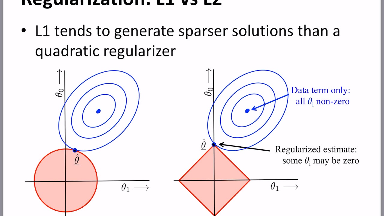
As the image illustrates, the circular L2 boundary is smooth, so the intersection is unlikely to occur exactly on an axis. In contrast, the L1 diamond has "pointy" corners that lie on the axes. It is geometrically much more likely that the loss contours will first make contact with the L1 constraint region at one of these corners, forcing one of the corresponding weights to be exactly zero. In higher dimensions, these "corners" become more numerous, leading to even greater sparsity.

This video provides a fantastic, detailed walkthrough of this geometric view and other properties of L1 and L2 regularization.

Optimization and Probabilistic Views

A crucial practical detail is that the L1 norm, $|w|$, is not differentiable at $w=0$. This means we cannot use standard gradient descent directly. This problem is typically solved using more advanced techniques like coordinate descent or subgradient methods, which are designed to handle such "kinks" in the objective function.

Furthermore, we can connect these regularizers to our study of probability. In a Bayesian framework, placing a prior distribution on the model's weights and performing Maximum A Posteriori (MAP) estimation is equivalent to regularized optimization.

• L2 Regularization is equivalent to placing a Gaussian prior ($\mathcal{N}(0,{\sigma }^2)$) on the weights. The smooth bell curve of the Gaussian encourages weights to be small but doesn't strongly favor values at exactly zero.
• L1 Regularization is equivalent to placing a Laplace prior on the weights. The Laplace distribution has a sharp peak at zero, which probabilistically expresses a stronger belief that weights should be exactly zero, thus encouraging sparsity.

Early Stopping: Regularization Through Time

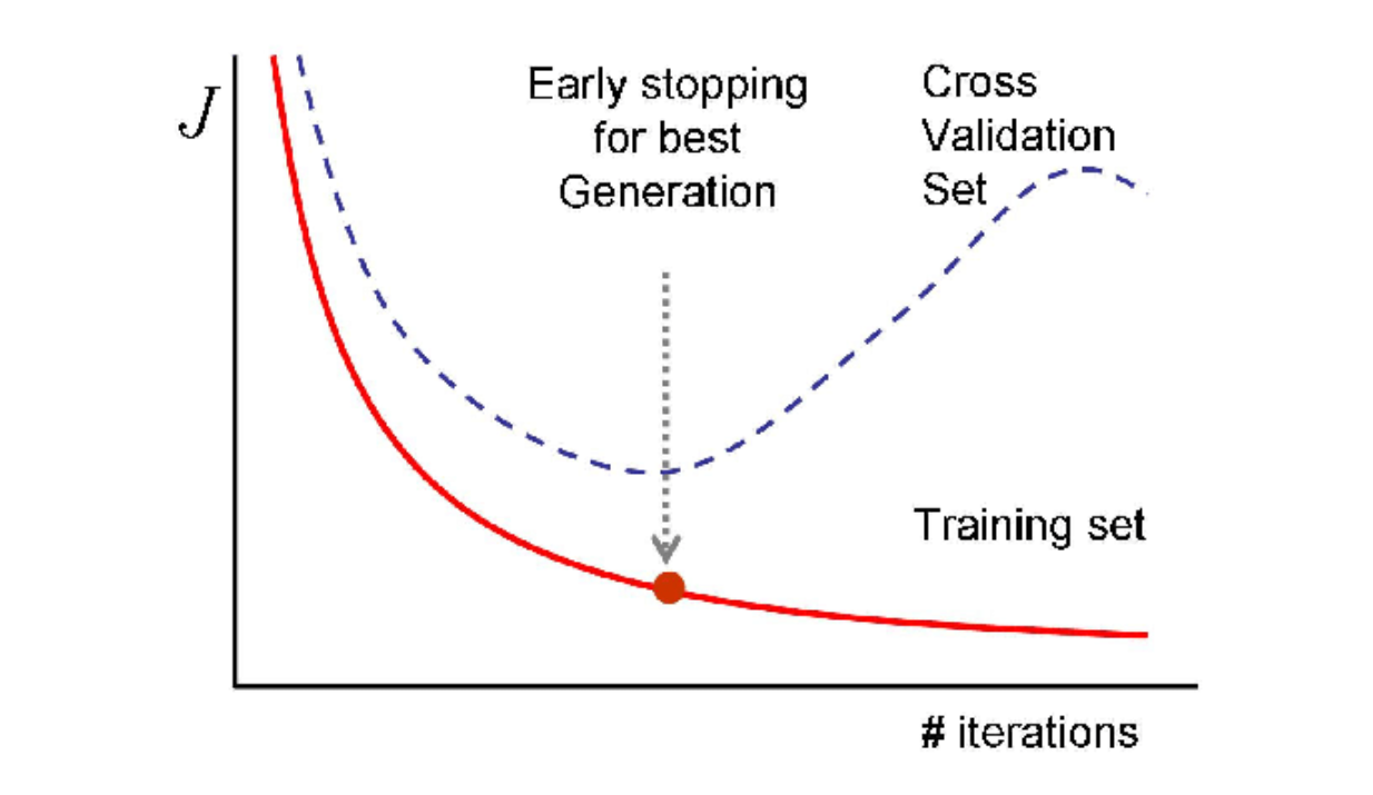
Early stopping is a strikingly different form of regularization. It doesn't alter the loss function or add any penalty terms. Instead, it is a procedural regularizer that leverages the validation set to decide when to halt the training process.

The intuition is straightforward:

1. As we train a model, we monitor its performance on both the training set and a separate validation set.
2. Initially, both training loss and validation loss will decrease.
3. However, after a certain point, the model will begin to overfit the training data. While the training loss continues to decrease, the validation loss will plateau and then start to increase. This is the moment the model begins to lose its ability to generalize.
4. Early stopping consists of saving the model weights at the epoch where the validation loss was at its minimum and halting the training process shortly after it starts to degrade.

The Hidden Link to L2 Regularization

This simple procedure seems purely heuristic, but it has a deep mathematical connection to L2 regularization. For a simple linear model with a quadratic error function, it can be shown that early stopping is mathematically equivalent to L2 regularization.

Let's build the intuition:

• Weight parameters are typically initialized to small values, often at or near the origin ($\mathbf{w}\approx 0$).
• During gradient descent, the weights move away from the origin into the parameter space to minimize the loss. The number of training steps, $\tau$, directly determines how far the weights can travel from their starting point.
• Stopping the training process early (using a small $\tau$) effectively confines the weight vector ${\mathbf{w}}^{(\tau )}$ to a small region around the origin.
• This is analogous to L2 regularization, which explicitly constrains the weights to a hypersphere of a certain radius. A smaller number of training steps in early stopping corresponds to a smaller radius (stronger regularization), while more training steps allow for a larger radius (weaker regularization).

Therefore, the number of training iterations $\tau$ in early stopping plays a role similar to the inverse of the regularization hyperparameter $\lambda$ in L2 regularization.

Conclusion

In this lesson, we've added two more powerful regularization techniques to our conceptual arsenal, moving beyond the standard L2 weight decay.

Key Takeaways:

• L1 Regularization (Lasso): Adds a penalty based on the sum of absolute weight values ($||\mathbf{w}|{|}_1$). Its primary advantage is inducing sparsity, effectively zeroing out the weights of less important features and performing implicit feature selection. Geometrically, this arises from the sharp "corners" of its diamond-shaped constraint region. Probabilistically, it corresponds to a Laplace prior on the weights.
• Early Stopping: A procedural regularizer that monitors validation performance and stops training when generalization error begins to increase. It is simple to implement and avoids the need for a regularization hyperparameter $\lambda$.
• Equivalence: For simple quadratic objectives, early stopping is mathematically equivalent to L2 regularization. The number of training steps plays a role analogous to the regularization strength.

Preview of the Next Lesson:

We have now concluded our comprehensive study of the fundamental principles and tools for training general-purpose deep neural networks. We are equipped with a robust understanding of optimization, backpropagation, and a variety of regularization methods.

With this foundation secure, we will pivot to the first of our specialized architectures, designed explicitly for visual data. In the next module, we will dive into Convolutional Neural Networks (CNNs). We'll start by connecting the convolution operation to its roots in classical image processing and then build up the architecture of modern CNNs, laying the groundwork for our future exploration of cutting-edge neural rendering techniques.