Recommended resources
The freely available resources this lesson will direct you to.
- Types of Fact Tables in Data Warehouse | Transaction, Periodic and Accumulatingwww.youtube.com
- 14 Transactional Fact Table and Periodic Snapshot Fact Tablewww.youtube.com
- Design Tip #167 Complementary Fact Table Types - Kimball Groupwww.kimballgroup.com
- Fact Tables and Dimension Tables - Kimball Groupwww.kimballgroup.com
Hello! This module moves beyond choosing a fact-table type and asks how to make that choice reliable in an analytical model. Earlier in the course, you defined grains and classified measures by additivity. Here you will use both skills to design a periodic snapshot for inventory, then specify how its balances may—and may not—be rolled up.
The practical test is simple: a dashboard asks for inventory by warehouse, quarter, and year. A well-designed snapshot can answer all three views without presenting the sum of twelve month-end balances as “year-end inventory.”
A snapshot measures a state, not a movement
Suppose an inventory system records receipts, shipments, and adjustments. Those are movements: summing their signed quantities over a period gives a net change. A manager may instead ask, “How many units were on hand at the end of March?” That is a question about state at a specified time.
A periodic snapshot records that state at regular intervals. It need not contain one row per movement, and its measurements need not be the sum of movements during the interval. If there were no movements today, today’s closing balance can still be important—and can still have a row.
Kimball Group’s Design Tip #167: Complementary Fact Table Types uses a logistics pipeline to show why movement transactions and inventory snapshots answer different questions.
Design Tip #167 Complementary Fact Table Types - Kimball Group
Read Kimball Group’s explanation of the periodic snapshot to distinguish inventory level from movement volume.
In the subsection “Periodic Snapshot Fact Table,” begin with the sentence “The second requirement is understanding the total amount of inventory at any point in the pipeline.” Read the snapshot explanation through the sentence about the two fact tables supporting the logistics pipeline. Focus on the stated row grain—one vehicle per day—and on the role of location. Stop before the following “Accumulating Snapshot Fact Table” subsection.
The source uses an individually identifiable vehicle as its inventory unit. For a warehouse holding interchangeable units, one row per product, location, and day is often more useful: that row contains the closing count for that combination. These are two legitimate grains for different inventory questions; they should not be mixed in one fact table.
Declare the row before choosing its columns
Consider this grain declaration:
One row records the quantity of one product at one warehouse at the close of one business day.
Every phrase constrains the design. One product determines the product key and unit of measure. One warehouse determines the location key. Close of one business day determines the snapshot date and cutoff rule. At this grain, an inventory fact might have these columns:
| Column | Purpose |
|---|---|
snapshot_date_key |
The business date whose closing state was measured |
product_key |
The product represented by the row |
warehouse_key |
The warehouse holding that product |
quantity_on_hand |
Units physically on hand at the defined cutoff |
inventory_value |
Optional value of those units under a documented valuation rule |
The date, product, and warehouse keys identify the dimensional context. The three-key combination should represent at most one closing observation; the load must not silently retain two versions of the same product–warehouse–day balance. If a correction arrives, its replacement or restatement policy needs to be explicit.
The phrase “quantity on hand” also needs a business definition. Does it include reserved stock? Damaged stock? Goods in transit? Two reports cannot be reconciled merely because both columns have the same name. Likewise, an inventory_value fact is useful only if its currency, valuation method, and cutoff match the intended analysis.
A monthly account-balance snapshot follows the same pattern but has a different grain: one account’s closing balance at the end of one month. You would substitute an account key for the product and warehouse keys, and define precisely what “month-end” means. Do not put monthly balances beside daily balances as interchangeable rows in the same fact table.
The semi-additive rule
A snapshot balance is semi-additive: you can usually sum it across appropriate non-time dimensions for the same instant, but not across snapshot dates.
Suppose the snapshot contains the following rows for one product:
| Closing date | Warehouse A | Warehouse B | Combined units |
|---|---|---|---|
| March 31 | 190 | 10 | 200 |
| June 30 | 184 | 12 | 196 |
March’s combined closing stock is units. June’s is units. But units is not the closing stock for either quarter or for the half-year. It adds two observations of substantially the same stock at different times.
For a set of warehouses and one agreed snapshot date , the valid total is:
If the question is closing balance for a quarter, select the quarter’s closing snapshot and then sum its warehouse rows. If the question is average daily inventory during a quarter, average the daily same-date totals, subject to the coverage and weighting rules discussed below. These are different metrics, not alternative labels for a time-sum.
This pivot-table image makes the reporting hazard visible:
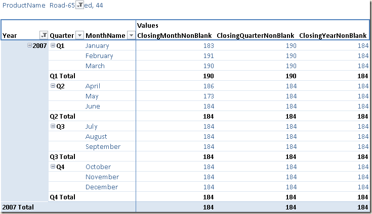
Notice that a quarterly or yearly closing figure represents the balance at the end of that period. A BI tool’s default “sum” subtotal cannot infer this rule from the numeric data type.
For a short visual treatment, watch the point-in-time portion of 14 Transactional Fact Table and Periodic Snapshot Fact Table from Ease With Data.
14 Transactional Fact Table and Periodic Snapshot Fact Table
Watch the point-in-time subscriber-count example to reinforce why a closing state is not summed across months.
Watch the snapshot example. Follow the January, February, and March totals, particularly the distinction between subscribers gained during a month and subscribers present at its end. Stop after the explanation that January, February, and March closing counts should not be added together.
The same distinction holds for stock: receipts during March are a flow; stock at March close is a balance.
Define each permitted aggregation
Your metric definition should tell a SQL author or BI-model author what to do along each axis. For quantity_on_hand, a reasonable contract is:
| Requested analysis | Rule |
|---|---|
| Multiple warehouses, one product, one snapshot date | Sum, provided warehouse populations do not overlap |
| Multiple products, one snapshot date | Sum units only when a combined-unit count is meaningful; otherwise retain product or unit-of-measure groupings |
| Quarter-end or year-end stock | Use the balance on the common closing date for that period |
| Average inventory over a period | Average balances at the specified observation frequency; document missing dates and weighting |
| Change between two dates | Subtract the earlier closing balance from the later one |
| Sum of daily or monthly closing balances | Do not label it inventory on hand |
The qualification “common closing date” matters. Selecting each warehouse’s latest available row independently could combine Warehouse A as of June 30 with Warehouse B as of June 27. That result describes no single point in time. For a quarter-end report, require complete June 30 coverage or clearly label and govern an alternative as-of policy.
Kimball Group’s Fact Tables and Dimension Tables introduces additivity and discusses averaging semi-additive balances over time.
Fact Tables and Dimension Tables - Kimball Group
Read Ralph Kimball’s explanation of additive versus semi-additive facts to connect the inventory rule to the broader dimensional-modeling principle.
In the “Additive Facts” subsection, start at “At the heart of every fact table is the list of facts that represent the measurements.” Read the additivity discussion through the explanation of dividing accumulated balances by the number of time periods, then finish the short final sentence naming “averaging over time.” Concentrate on why balances differ from sales amounts.
Averaging needs a defined denominator. With one complete, equally weighted daily observation per date, the arithmetic mean of daily closing totals is an average daily closing balance. With one observation per month, averaging twelve month-end balances produces an average of month-end balances—not necessarily the same as a daily average. Missing days must not silently shrink the denominator, and uneven intervals may call for a time-weighted average instead. Neither average should be presented as “year-end stock.”
Make the rule visible in queries and the semantic layer
Your SQL experience makes a useful implementation check possible without designing the full PostgreSQL load yet. Assume fact_inventory_daily contains the declared product–warehouse–day rows, and dim_date marks calendar quarter-end dates.
A quarter-end stock query deliberately filters to the closing date before summing:
SELECT
    d.calendar_year,
    d.calendar_quarter,
    f.product_key,
    SUM(f.quantity_on_hand) AS quarter_end_units
FROM fact_inventory_daily AS f
JOIN dim_date AS d
  ON d.date_key = f.snapshot_date_key
WHERE d.is_calendar_quarter_end = TRUE
GROUP BY
    d.calendar_year,
    d.calendar_quarter,
    f.product_key;
This query is correct only if every warehouse expected in the total has a row for that same quarter-end date, and the product’s units are compatible. A production design should check that coverage before publishing the result. Changing is_calendar_quarter_end to a year-end indicator would produce year-end balances; removing the date filter and summing all rows would not.
For a daily average, the semantic intent is different: first obtain one total per date across the relevant warehouses, then average those daily totals. Its label should say average daily closing units, not closing units. A BI semantic model should likewise expose distinct, explicitly named measures for quarter-end balance and average balance rather than allowing a generic sum over the date hierarchy.
Sparse days, zero stock, and data freshness
The row policy is part of the model, not just an ETL detail. If the declared grain is every active product–warehouse combination every day, write a row with quantity_on_hand = 0 when stock is confirmed to be zero. No row means something else: the product was outside the snapshot’s coverage, the source did not report, or the load failed. Those cases require investigation or an explicit business rule; they must not automatically become zeros.
Daily snapshots also have an as-of cutoff. A warehouse closing at local business-day end and another closing at a different cutoff cannot be safely totaled without a stated synchronization policy. Record the snapshot date and cutoff convention in metric metadata, and monitor load completeness and freshness. If late adjustments restate an earlier day, decide whether reports use corrected history and ensure any quarter-end summaries are updated consistently.
These controls preserve the semi-additive rule in practice. A mathematically correct SUM across warehouses is still misleading if one warehouse is absent, counted twice, or measured at a different time.
Closing perspective
A periodic snapshot starts with a precise state-at-time grain: for example, one product, one warehouse, one closing business day. Its inventory or account balance can be summed across compatible entities at that same time. Across time, choose the appropriate closing observation, calculate a clearly defined average, or calculate a change—never treat a sum of balances as closing stock.
In the next lesson, you will use a different snapshot pattern to follow a process through milestone dates. The distinction to retain is that this lesson’s periodic rows represent repeated states at regular cutoffs, rather than one process instance progressing through its lifecycle.