The Training Objective of DDPMs

Hello! Welcome back to our exploration of diffusion models.

In the previous lesson, we established the core intuition behind diffusion models: a forward process that systematically destroys an image with noise, and a reverse process where a neural network learns to undo this destruction to generate a new image. We learned that the model's task is to predict the noise that was added at any given step.

Today, we will dive into the mathematics that make this training possible. Our goal is to answer the question: What is the exact objective function that the model minimizes? This lesson directly addresses the learning outcome: Describe the training objective of a denoising diffusion probabilistic model (DDPM).

We will start from a high-level, statistically-grounded goal and see how the authors of the original DDPM paper ingeniously simplified it into a straightforward and effective loss function. Given your background in mathematics, you'll find the derivation from a complex probabilistic objective to a simple Mean Squared Error loss particularly interesting.

1. The Ideal but Intractable Objective

From a statistical perspective, the goal of any generative model is to learn the true data distribution $p(x)$. A standard way to achieve this is to train a parameterized model $p_{\theta }(x)$ to maximize the likelihood of the training data. For a single data sample $x_0$, we want to maximize $p_{\theta }(x_0)$. In practice, we minimize the negative log-likelihood (NLL):

However, for diffusion models, calculating $p_{\theta }(x_0)$ is intractable. To get the probability of a specific clean image $x_0$, we would have to consider every possible path of denoising steps that could have led to it, starting from pure noise. This involves integrating over all possible latent variables $x_1,\dots ,x_T$, which is computationally impossible.

This is where a common technique in variational inference comes to the rescue.

2. From Log-Likelihood to the Evidence Lower Bound (ELBO)

Since we can't optimize the log-likelihood directly, we optimize a lower bound on it instead. This is called the Evidence Lower Bound (ELBO), or sometimes the Variational Lower Bound (VLB). By maximizing the ELBO, we are guaranteed to be pushing up the actual log-likelihood.

The derivation of the ELBO is a cornerstone of modern generative modeling, including VAEs, which you might recall. The following video provides a step-by-step walkthrough of how we arrive at the ELBO for diffusion models and begin to simplify it.

After this derivation, we are left with a loss function composed primarily of a sum of KL divergence terms:

Let's break down what this means.

• $p_{\theta }(x_{t-1}|x_t)$ is our learned reverse step. It's what our neural network is trying to approximate: how to go from a noisy image $x_t$ to a slightly less noisy image $x_{t-1}$.
• $q(x_{t-1}|x_t,x_0)$ is the true posterior of the reverse step. Crucially, this is the true distribution for the reverse step if we know the original image $x_0$.

So, the objective is to train our network $p_{\theta }$ to match the true reverse distribution $q$, which we can calculate during training because we have $x_0$.

3. The Final Simplification: A Mean Squared Error Loss

The KL divergence measures the "distance" between two probability distributions. Our objective is to make our learned reverse distribution $p_{\theta }$ as close as possible to the true posterior $q$.

It turns out that both of these distributions are Gaussian. A key simplification in the DDPM paper is to fix the variance of our learned distribution $p_{\theta }$ and only have the neural network predict its mean, ${\mu }_{\theta }(x_t,t)$.

When you calculate the KL divergence between two Gaussian distributions with the same variance, it simplifies to the squared distance between their means!

This transforms our loss into minimizing the L2 distance between the mean of the true posterior and the mean predicted by our network.

The final, brilliant step is to reparameterize both means in terms of the noise, $ϵ$. This reveals that many complex terms cancel out, leaving us with an incredibly simple final objective. Let's watch the conclusion of the derivation.

As the video concludes, the complex ELBO objective simplifies to:

where $x_t=\sqrt{{\bar{\alpha }}_t}{x}_0+\sqrt{1-{\bar{\alpha }}_t}ϵ$.

This is the training objective of a DDPM. In plain English:

1. Pick a random clean image $x_0$ from your dataset.
2. Pick a random timestep $t$.
3. Generate a random noise tensor $ϵ$.
4. Create the noisy image $x_t$ using the forward process formula.
5. Feed $x_t$ and $t$ into your neural network (the U-Net) to get its noise prediction, ${ϵ}_{\theta }$.
6. Calculate the Mean Squared Error (MSE) between the actual noise $ϵ$ and the predicted noise ${ϵ}_{\theta }$.
7. Update the model's weights using this loss.

The following diagram beautifully illustrates the training algorithm, highlighting the simplified loss function at its core.

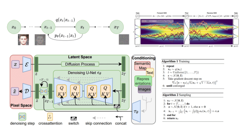
To reinforce this, let's watch one more short clip that describes the training loop from a more practical coding perspective.

4. Why Predict Noise?

A natural question is: why go to the trouble of predicting the noise $ϵ$ instead of just predicting the clean image $x_0$ directly?

Predicting the noise turns out to be a much better-conditioned problem.

• At high noise levels (large $t$), the image is mostly noise. Predicting the original clean image $x_0$ is nearly impossible, as the signal is lost. However, predicting the noise $ϵ$ is relatively straightforward because it's the dominant component.
• At low noise levels (small $t$), the image is mostly clean. Predicting the noise is still a well-defined task (predicting a small-magnitude noise vector), whereas other objectives can have issues.

This "epsilon objective" provides a stable learning signal across all timesteps, which is a key reason for the success of DDPMs.

Conclusion

In this lesson, we traced the path from a foundational principle of generative modeling—maximizing data likelihood—to the concrete and simple training objective used in DDPMs.

Key Takeaways:

• The ideal objective of maximizing log-likelihood is intractable for diffusion models.
• We instead optimize a tractable surrogate, the Evidence Lower Bound (ELBO).
• The ELBO can be expressed as a sum of KL divergence terms, which measure the distance between our learned reverse process and the true (but unusable for inference) reverse process.
• The key simplification in the DDPM paper is to show that this complex objective reduces to a simple Mean Squared Error (MSE) loss.
• The final training objective is to minimize the squared difference between the actual noise added to an image and the noise predicted by the neural network.

Preview of the Next Lesson

We have now covered the core theory: the forward/reverse processes and the training objective. In the next lesson, we'll put this theory into practice. You will learn how to use a pre-trained diffusion model (like Stable Diffusion) to generate images from text prompts, moving from the "how it works" to the "how to use it."