Encoding Cyclical Time with Sine/Cosine Transformations

Recommended resources

The freely available resources this lesson will direct you to.

In our previous lesson, we explored how to extract valuable information from a time series's own history using lag, rolling, and expanding window features. These techniques are powerful for capturing momentum and trends based on the target variable itself. Now, we shift our focus from the values in the time series to the timestamps at which they occur.

This lesson addresses a subtle but critical challenge in time series modeling: how to represent cyclical patterns like the hour of the day or the month of the year. A naive numerical encoding can mislead your model, but a clever transformation can unlock significant predictive power. We will explore how to use sine and cosine functions to encode cyclical temporal features, ensuring that the model understands the continuous, wrapping nature of time.

The Midnight Paradox: Why Linear Time Fails

Many machine learning models, particularly those based on linear relationships or distance metrics (like linear regression, SVMs, or KNN), interpret numerical features as being on a continuous, monotonic scale. For these models, a larger number means "more" of something.

Consider the 'hour of the day' feature, which we might encode as integers from 0 to 23. To a model, the distance between hour 23 (11 PM) and hour 0 (midnight) is 23 units, the largest possible gap. In reality, they are only one hour apart. This is the "midnight paradox," and it causes models to see an artificial discontinuity where none exists.

The following article offers an excellent introduction to this problem and why common approaches fall short.

Is Your Model Time-Blind? The Case for Cyclical Feature ...

This article from Towards Data Science clearly frames the problem of encoding cyclical features.

Read the introduction, which vividly explains the core issue. Then, continue to the next section, The Failure of Standard Encoding, which discusses the limitations of both simple numerical encoding and one-hot encoding for time-based features.

As the article points out, one-hot encoding can solve the discontinuity problem, but it does so at the cost of increasing dimensionality and, more importantly, losing all information about proximity. With one-hot encoding, hour 2 is no closer to hour 3 than it is to hour 10. We need a method that preserves both continuity and proximity.

The Solution: Mapping Time to a Circle

The most elegant solution is to stop thinking of time as a line and start thinking of it as a circle. An hour on a clock, a day in a week, or a month in a year are all points on a cycle. We can represent any point on a circle using two coordinates, an $x$ and a $y$ value, derived from sine and cosine functions.

This diagram illustrates the core concept: a linear feature like 'hour of the day' is transformed into a cyclical one, where hour 23 is naturally adjacent to hour 0, just like on a clock face.

For a given time variable t with a period P (e.g., 24 for hours, 7 for days of the week), we can generate two new features:

feature_{s i n} = sin (\frac{2 π t}{P})

feature_{c o s} = cos (\frac{2 π t}{P})

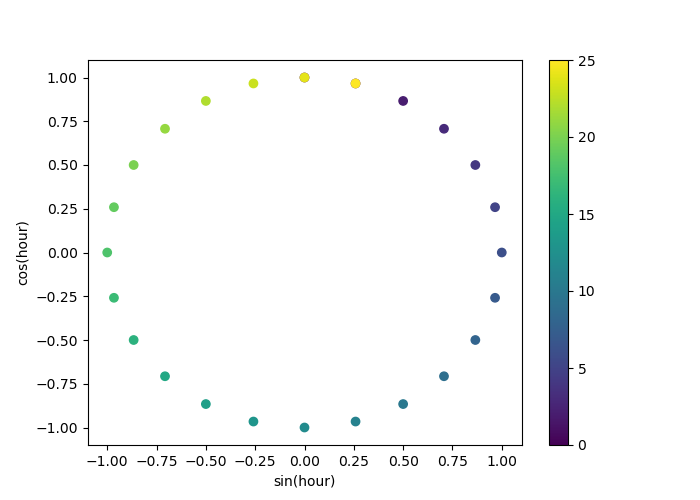
These two features together give each point in the cycle a unique coordinate in a 2D space. The beauty of this is that points that are close in time will also be close in this new 2D feature space. For example, hour 23 and hour 0 will have very similar (x, y) coordinates.

The following resource from the scikit-learn documentation provides a fantastic visualization and a practical implementation.

Time-related feature engineering

This scikit-learn example demonstrates cyclical feature engineering and provides clear code and visualizations.

Please read the section titled Trigonometric features. Focus on the Python code that defines sin_transformer and cos_transformer, and carefully examine the resulting 2D scatter plot. This plot is the key to understanding the transformation.

The circular scatter plot from that example is shown below. Notice how the hours are arranged in a circle, with 0 and 23 adjacent to each other. The color gradient shows the original hour value, clearly illustrating the continuous loop.

This scatter plot shows the result of transforming the 'hour' feature. Each point's position is determined by its sin(hour) and cos(hour) values, forming a perfect circle. The color indicates the original hour, showing how hour 23 (dark purple) is now spatially close to hour 0 (also dark purple).

Why Both Sine and Cosine?

You might be tempted to use only one of the two functions to save a feature. However, this would introduce ambiguity. For example, on a 24-hour cycle, sin(6) (6 AM) has the same value as sin(18) (6 PM). The model would be unable to distinguish between these two very different times. Using both sine and cosine provides a unique (x, y) coordinate for every point in the cycle, resolving this ambiguity. The Towards Data Science article you read earlier makes this point well.

Is Your Model Time-Blind? The Case for Cyclical Feature ...

Let's revisit this article to solidify a few key points.

Read the section Why You Need Both Sine and Cosine for a clear explanation of this critical detail. Also, review the following section, Real-World Impact & Results, which discusses how this encoding benefits different model types, including the tree-based models you are familiar with.

Deeper Connections: Fourier Series and Periodicity

This sine/cosine transformation is not just a clever trick; it has a firm mathematical basis. It is, in fact, an application of a first-order Fourier series. A Fourier series decomposes a periodic function into a sum of simple sine and cosine waves. By using the fundamental frequency (e.g., one cycle per 24 hours), we are essentially fitting the simplest possible periodic model to our time feature.

This connection becomes especially important when dealing with real-world data, where defining the period P correctly is paramount. The following video on modeling seasonality provides a brilliant example of this.

This video from the QuantPy channel discusses modeling seasonality using Fourier series and contains an invaluable lesson on defining the period correctly.

First, watch the brief introduction from the beginning to understand the context of time series decomposition. Then, watch the section from modeling seasonality, which introduces the Fourier series and shows how a first-order sine and cosine pair can model the main seasonal component. Finally, and most importantly, pay close attention to the segment from the phase shift problem. The speaker discovers their model is drifting because they used a period of 365 days, ignoring leap years. Changing the period to 365.25 solves the problem. This is a perfect example of the precision required for robust temporal feature engineering.

This detail about the period (365 vs. 365.25) is precisely the kind of low-level detail that separates a quick prototype from a production-grade system that remains accurate over long time horizons. For financial data, correctly accounting for trading days versus calendar days, or handling complex fiscal year calendars, can be similarly crucial.

Interview Alert: You are building a model to predict trading volume for a specific stock. Your features include the timestamp of each trade. How would you represent the 'time of day' and 'day of week' as features for a gradient boosting model, and why is your approach superior to simpler methods?

A strong answer would be:

Identify Cyclical Nature: State that 'time of day', 'day of week', and 'month of year' are cyclical features.

Propose Sine/Cosine Encoding: Explain that you would transform each cyclical feature into two new features using sine and cosine transformations with the appropriate period (e.g., 24 for hour, 7 for day of week).

Justify the Approach:

vs. Linear Encoding: It avoids the "midnight paradox," correctly representing that 11 PM is close to midnight, which is crucial for capturing patterns around market open and close.

vs. One-Hot Encoding: It preserves proximity information and does so with only two features, avoiding the high dimensionality and potential for overfitting that one-hot encoding can cause, especially for features with many levels (like minute of the day).

For Tree Models: Acknowledge that while powerful tree-based models can eventually learn the non-linear relationship from a simple linear feature by making many splits, providing cyclical features explicitly makes the model's job easier. It allows the model to learn smoother decision boundaries related to time, often leading to better performance and faster convergence with fewer, shallower trees.

Conclusion

In this lesson, you've moved beyond engineering features from the time series values to engineering them from the timestamps themselves. By understanding the limitations of naive temporal representations, you can now build models that correctly interpret the cyclical nature of time.

Key Takeaways:

The Problem: Representing cyclical features like 'hour of day' with a simple linear encoding creates artificial discontinuities that can harm model performance.
The Solution: Sine and cosine transformations map a single cyclical feature onto a 2D space, preserving the proximity of boundary values (e.g., December and January).
Implementation: This requires creating two features for each original cyclical feature. It's crucial to use both sine and cosine to avoid ambiguity.
Mathematical Foundation: This technique is a practical application of a first-order Fourier series, used to model the primary frequency of a cycle.
Practical Precision: The accuracy of the encoding depends on choosing the correct period (e.g., 365.25 for yearly patterns to account for leap years), a detail that is critical for long-term model stability.

Having mastered how to encode predictable, repeating cycles, our next lesson will address the opposite: detecting and encoding abrupt, unpredictable shifts in a time series. We will explore statistical methods for identifying structural breaks and regime changes, allowing you to turn these critical events into powerful features for your models.