Modeling Phase Transitions with φ⁶ Theory

Recommended resources

The freely available resources this lesson will direct you to.

Hello! Welcome back to our study of phase transitions.

In the last lesson, we successfully used the $ϕ^{4}$ Landau theory to derive the full set of mean-field critical exponents ( $α = 0$ , $β = 1/2$ , $γ = 1$ , $δ = 3$ ). We saw that this theory, with its positive quartic coefficient ( $b > 0$ ), provides an excellent description of continuous (second-order) transitions, where the order parameter grows smoothly from zero.

However, many common phase transitions, like boiling water or melting ice, are first-order: the order parameter (e.g., the difference in density between liquid and gas) jumps discontinuously at the transition temperature. Today, we'll extend Landau theory to model these phenomena. Our goal is to use $ϕ^{6}$ theory to model first-order transitions and locate the tricritical point. We will see how a change in a single coefficient can alter the fundamental nature of the transition, and we'll identify the special point in the phase diagram where a continuous transition line meets a first-order one.

1. Modeling First-Order Transitions

A first-order transition is characterized by a discontinuous change in the order parameter, $η$ . Within Landau theory, this occurs when the global minimum of the free energy jumps from one value to another as a parameter (like temperature) is varied. This can happen in two primary scenarios.

Scenario 1: No Inversion Symmetry (A Cubic Term)

In our $ϕ^{4}$ model, the $m \to - m$ symmetry was crucial. If the underlying physics doesn't possess this symmetry, the Landau expansion can include odd powers of the order parameter. The simplest such case includes a cubic term:
$f (η) = f_{0} + \frac{1}{2} a η^{2} - \frac{1}{3} y η^{3} + \frac{1}{4} b η^{4}$
Here, we assume $y > 0$ and $b > 0$ for stability. The negative sign on the cubic term is a convention; if $y$ were negative, we could flip the sign of $η$ . This cubic term breaks the $η \to - η$ symmetry and favors a positive order parameter.

To understand the behavior, let's analyze the minima of $f (η)$ .

7.5: Landau Theory of Phase Transitions - Physics LibreTexts

The following text from 'Physics LibreTexts' by Daniel Arovas provides a concise mathematical analysis of a Landau theory with a cubic term. It shows how this term leads to a first-order transition.

Please read the subsection titled 'Cubic terms in Landau theory : first order transitions'. Focus on how the analysis identifies the conditions under which there are multiple minima and how the transition point is found by setting the free energies of these minima equal.

As the text explains, the key is the competition between the quadratic term, which favors $η = 0$ when $a > 0$ , and the cubic term, which favors $η > 0$ .

For high temperatures ( $a$ is large and positive), the quadratic term dominates, and the only minimum is at $η = 0$ .
As temperature decreases ( $a$ decreases), another local minimum appears at a positive value of $η$ . For a range of $a$ , the $η = 0$ state is still the global minimum (it's metastable).
The first-order transition occurs at a specific temperature $T_{c}$ (corresponding to $a_{c} = 2 y^{2} /9 b$ ) where the free energy of the new minimum becomes equal to the free energy of the $η = 0$ minimum.
At this point, the order parameter jumps discontinuously from $η = 0$ to $η_{c} = 2 y /3 b$ . The second-order transition that would have happened at $a = 0$ is preempted by this first-order jump.

Scenario 2: With Inversion Symmetry ( $ϕ^{6}$ Theory)

What if the system does have $η \to - η$ symmetry, but still undergoes a first-order transition? This can happen if the coefficient of the $η^{4}$ term, $b$ , is negative. A negative $b$ would make the free energy decrease without bound for large $η$ , which is unphysical. To ensure stability, we must include the next-higher-order symmetric term:
$f (η) = f_{0} + \frac{1}{2} a η^{2} + \frac{1}{4} b η^{4} + \frac{1}{6} c η^{6}$
This is the $ϕ^{6}$ theory. We require $c > 0$ for stability ( $f \to \infty$ as $η \to \pm \infty$ ). The interesting physics arises when $b < 0$ .

The shape of this free energy potential is key. For $b < 0$ and small, positive $a$ , the potential develops two new minima at $η \neq = 0$ , in addition to the local minimum at $η = 0$ .

Potential Energy Landscape for a First-Order Phase Transition — Evolution of the potential energy $V(\rho)$ (equivalent to our free energy $f(\eta)$) as a function of the order parameter $\rho$ for different values of a control parameter $\tau$ (equivalent to temperature or our coefficient $a$). For $\tau > \tau_1$ (high temperature), there is a single minimum at $\rho=0$. For $\tau < \tau_1$ (lower temperature), a double-well potential develops, characteristic of the $\phi^6$ theory with $b<0$.

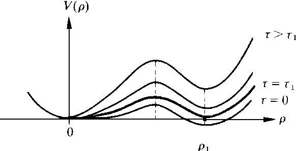
To find the transition point, we follow the same logic as before: the first-order transition occurs when the non-zero minima have the same free energy as the minimum at $η = 0$ . This requires solving two simultaneous equations:

$\frac{\partial f}{\partial η} = η (a + b η^{2} + c η^{4}) = 0$ (The equilibrium condition)
$f (η) - f (0) = \frac{1}{2} a η^{2} + \frac{1}{4} b η^{4} + \frac{1}{6} c η^{6} = 0$ (The equal-energy condition)

Solving this system (for $η \neq = 0$ ) gives the condition for the first-order phase transition line:
$a_{c} = \frac{3 b ^{2}}{16 c} (for b < 0)$
At this transition, the order parameter jumps from $η = 0$ to $η_{c}^{2} = - \frac{3 b}{4 c}$ . Since this transition occurs at a positive value of $a_{c}$ , it again preempts the continuous transition that would have occurred at $a = 0$ .

The following reading from Wikipedia confirms this result and provides additional context.

Landau theory - Wikipedia

The Wikipedia article on Landau theory has a good section on modeling first-order transitions, specifically for the symmetric case that leads to the φ⁶ model.

Please read the subsection 'I. Symmetric Case' under 'First-order transitions'. It walks through the logic for the φ⁶ free energy and derives the conditions for the first-order transition temperature and the magnitude of the order parameter jump.

Test your understanding!

In the $ϕ^{6}$ model with $b < 0$ , consider the regime where $0 < a < b^{2} / (4 c)$ . In this regime, the equation $a + b η^{2} + c η^{4} = 0$ has two distinct positive solutions for $η^{2}$ . This means there are five real roots for $f^{'} (η) = 0$ : one at $η = 0$ and four at $\pm η_{1}, \pm η_{2}$ . Which of these correspond to local minima of the free energy?

Show answer

To determine stability, we examine the second derivative, $f^{''} (η) = a + 3 b η^{2} + 5 c η^{4}$ .

At $η = 0$ : $f^{''} (0) = a$ . Since we are in the regime $a > 0$ , the point $η = 0$ is a local minimum.
At the other roots: We can rewrite $f^{''} (η)$ using the fact that $a + b η^{2} + c η^{4} = 0$ . This gives $f^{''} (η) = 2 b η^{2} + 4 c η^{4} = 2 η^{2} (b + 2 c η^{2})$ . The sign of $f^{''}$ depends on the sign of $b + 2 c η^{2}$ .
- The larger roots $\pm η_{1}$ (where $η_{1}^{2} = \frac{- b + b ^{2} - 4 a c}{2 c}$ ) correspond to local minima because $b + 2 c η_{1}^{2} = b^{2} - 4 a c > 0$ .
- The smaller roots $\pm η_{2}$ (where $η_{2}^{2} = \frac{- b - b ^{2} - 4 a c}{2 c}$ ) correspond to local maxima because $b + 2 c η_{2}^{2} = - b^{2} - 4 a c < 0$ .

Therefore, there are three local minima ( $0, \pm η_{1}$ ) separated by two local maxima ( $\pm η_{2}$ ), creating the characteristic double-well potential shown in the figure above.

2. The Tricritical Point

We have now established two distinct behaviors based on the sign of $b$ in the $ϕ^{6}$ theory:

If $b > 0$ : The $η^{4}$ term is stabilizing. The $η^{6}$ term is irrelevant for small $η$ . We recover the $ϕ^{4}$ theory, which has a second-order (continuous) transition at $a = 0$ .
If $b < 0$ : The $η^{4}$ term is destabilizing. The $η^{6}$ term provides stability. This leads to a first-order (discontinuous) transition at $a = \frac{3 b ^{2}}{16 c} > 0$ .

Now, imagine we have a physical system where we can tune not only the temperature (which controls $a$ ) but also another parameter, like pressure or concentration, which controls the sign and magnitude of $b$ .

The tricritical point is the special point in the phase diagram where the character of the transition changes from second-order to first-order. It is the endpoint of a line of second-order transitions.

Looking at our conditions, this confluence occurs precisely when both transition conditions are met simultaneously:
$a = 0 and b = 0$

At the tricritical point, the Landau free energy expansion must be $f \approx \frac{1}{6} c η^{6}$ (since $a = b = 0$ ), making the potential at the critical point extremely flat. This leads to a unique set of critical exponents, different from the mean-field exponents we found earlier. For example, at the tricritical point, the order parameter scales with field as $η \sim h^{1/5}$ , so $δ_{TCP} = 5$ , which is different from the mean-field value $δ = 3$ .

The phase diagram in the $(b, a)$ parameter space neatly summarizes this:

The positive $a$ -axis corresponds to the disordered phase ( $η = 0$ ).
The positive $b$ -axis for $a = 0$ ( $a = 0, b > 0$ ) is a line of second-order critical points.
The curve $a = 3 b^{2} /16 c$ in the $b < 0$ half-plane is a line of first-order transitions.
The origin, $(a, b) = (0, 0)$ , where these two lines meet, is the tricritical point.

Conclusion

Key Takeaways:

First-order transitions, where the order parameter is discontinuous, can be modeled in Landau theory by either breaking the $η \to - η$ symmetry (adding a cubic term) or by having a negative quartic coefficient ( $b < 0$ ).
A negative $b$ necessitates a stabilizing sixth-order term, leading to the $ϕ^{6}$ model: $f = \frac{1}{2} a η^{2} + \frac{1}{4} b η^{4} + \frac{1}{6} c η^{6}$ .
In the $ϕ^{6}$ model, the sign of the coefficient $b$ determines the order of the transition.
The tricritical point $(a = 0, b = 0)$ is a special, higher-order critical point that separates a line of second-order transitions ( $b > 0$ ) from a line of first-order transitions ( $b < 0$ ).

Preview of the Next Lesson:

We have now developed the Landau formalism for continuous, first-order, and tricritical points using abstract $ϕ^{4}$ and $ϕ^{6}$ theories. The power of this approach lies in its generality. In our next lesson, we will see this in action as we apply Landau theory to model a specific physical system, such as a cubic-to-tetragonal structural transition in a crystal, connecting the abstract coefficients $a$ and $b$ to real material properties.