Data Modeling for Aggregated Token Counts

Hello! Welcome back to our course.

In our last lesson, we designed a resilient API to capture incremental usage reports from streaming LLM responses. We now have a reliable pipeline that pushes a stream of detailed usage events into a message queue. However, this raw event log, which could contain billions of entries, is not suitable for answering business-critical questions like "How much has this user spent this month?" without slow and expensive full-table scans.

Today, we'll address this by designing the data model that consumes these events. Our learning outcome is to design a data model for storing aggregated token counts that supports efficient querying by user, model, and time. We'll move from a simple event log to a read-optimized analytical store, a process you're likely familiar with from handling large-scale operational data at AWS.

1. The Need for Aggregation: From Raw Events to Actionable Insights

Querying a raw event log for analytics is inefficient for several reasons:

• High Volume: A system handling thousands of requests per second generates billions of events per month. Querying this volume on-the-fly is slow.
• Repetitive Computation: Calculating a user's monthly spend would require summing up millions of individual event records every single time the query is run.
• Cost: In most managed data systems, scanning large amounts of data is expensive.

The solution is pre-aggregation. We'll process the stream of raw events to compute summary statistics and store them in a read-optimized format. Instead of storing every single request, we'll store totals rolled up into time buckets.

Visually, we're aiming to build the data structures needed to generate reports like these, which summarize usage across different dimensions:

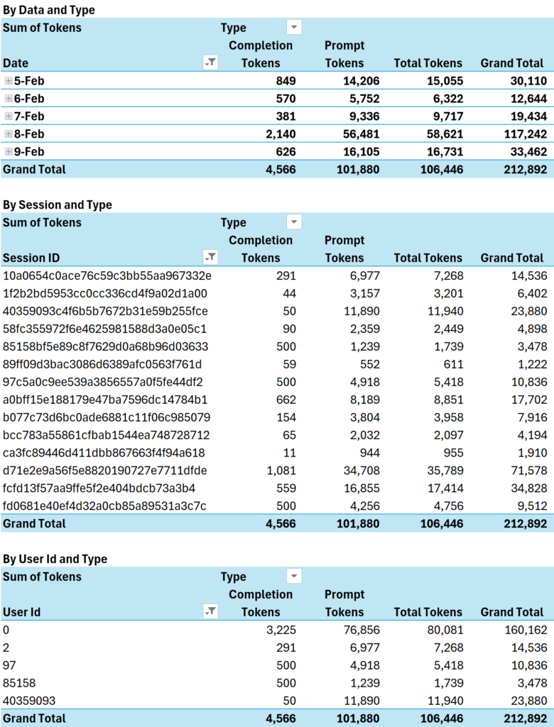
The key dimensions for our billing and analytics system are user, model, and time. Our data model must be indexed on these dimensions to allow for rapid filtering and retrieval.

2. Choosing the Right Datastore: A Game of Trade-offs

The choice of database is critical and depends entirely on the workload. Our workload is characterized by:

1. High-throughput writes: The system must absorb a constant stream of aggregation updates.
2. Time-series data: Usage is intrinsically ordered by time.
3. Analytical queries: We need to perform aggregations (SUM, AVG) over time ranges and filter by dimensions like user_id and model_id.

A standard relational database (like PostgreSQL) can struggle with this combination of high-volume writes and analytical queries at scale. This is a classic problem in observability and metrics systems.

A purpose-built Time-Series Database (TSDB) is often a perfect fit. To understand why, let's explore how they are designed.

As the video explains, TSDBs are optimized for this specific data shape. They use techniques like columnar storage, time-based partitioning, and compression to handle massive write volumes and execute time-series queries very quickly.

Another strong candidate is an Online Analytical Processing (OLAP) database or data warehouse, such as Amazon Redshift or Google BigQuery. These systems are designed for complex analytical queries over massive datasets and are a cornerstone of many data-intensive applications.

For our design, we'll consider both approaches as they are often used together in a hybrid architecture.

3. Designing the Aggregation Schema

Let's design a concrete schema for our aggregated data. We need to decide on the granularity of our time_bucket and the exact fields to store. A one-minute or one-hour granularity is a common starting point.

Schema for an OLAP Database (e.g., Amazon Redshift)

In a columnar data warehouse, a single wide table is often effective.

CREATE TABLE aggregated_token_usage (
    -- The beginning of the aggregation window (e.g., top of the hour)
    time_bucket_hourly TIMESTAMP NOT NULL,
    
    -- Dimensions for filtering
    tenant_id VARCHAR(256) NOT NULL,
    user_id VARCHAR(256) NOT NULL,
    model_id VARCHAR(128) NOT NULL,
    feature_id VARCHAR(128), -- e.g., 'summarizer', 'chatbot'

    -- Aggregated measures
    sum_input_tokens BIGINT NOT NULL,
    sum_output_tokens BIGINT NOT NULL,
    total_cost_usd DECIMAL(18, 9) NOT NULL, -- High precision for cost
    request_count INT NOT NULL,

    -- For Redshift, physical design is key.
    -- We distribute by tenant to keep a customer's data together.
    -- We sort by time to make time-range queries extremely fast.
    DISTKEY (tenant_id),
    SORTKEY (time_bucket_hourly, user_id)
);

Schema for a Time-Series Database (e.g., Amazon Timestream)

In a TSDB, the schema is defined by measurements, dimensions, and measures.

• Measurement Name: token_usage_metrics
• Dimensions (Tags): tenant_id, user_id, model_id, feature_id (used for filtering/grouping)
• Measures (Fields): input_tokens, output_tokens, cost_usd, request_count
• Timestamp: The timestamp of the aggregation bucket.

The key difference is conceptual: the OLAP model is a single table, while the TSDB model treats each unique combination of dimensions as a separate series.

A Critical Consideration: Cardinality
The number of unique dimension values (e.g., millions of user_ids) is called cardinality. High cardinality can be challenging for some TSDBs, as it creates millions of individual time series. This is a critical trade-off to consider when choosing a database and a data model. OLAP databases are generally more robust at handling high-cardinality dimensions.

4. Architectural Patterns for Aggregation

Now, how do we populate this aggregated table from the raw events in our message queue? The most robust, production-grade approach is a hybrid architecture (often called a Lambda or Kappa architecture) that combines stream and batch processing.

Inspired by the Netflix architecture, our system will have two main data flow paths:

1. The "Speed" Layer (Stream Processing)
This layer provides near real-time data for live dashboards.

• A stream processing engine (like Apache Flink or Kinesis Data Analytics) reads events from the message queue.
• It aggregates events in memory over short, "tumbling" time windows (e.g., one minute).
• At the end of each window, it writes the aggregated result to our database. This provides data with a latency of about one minute.

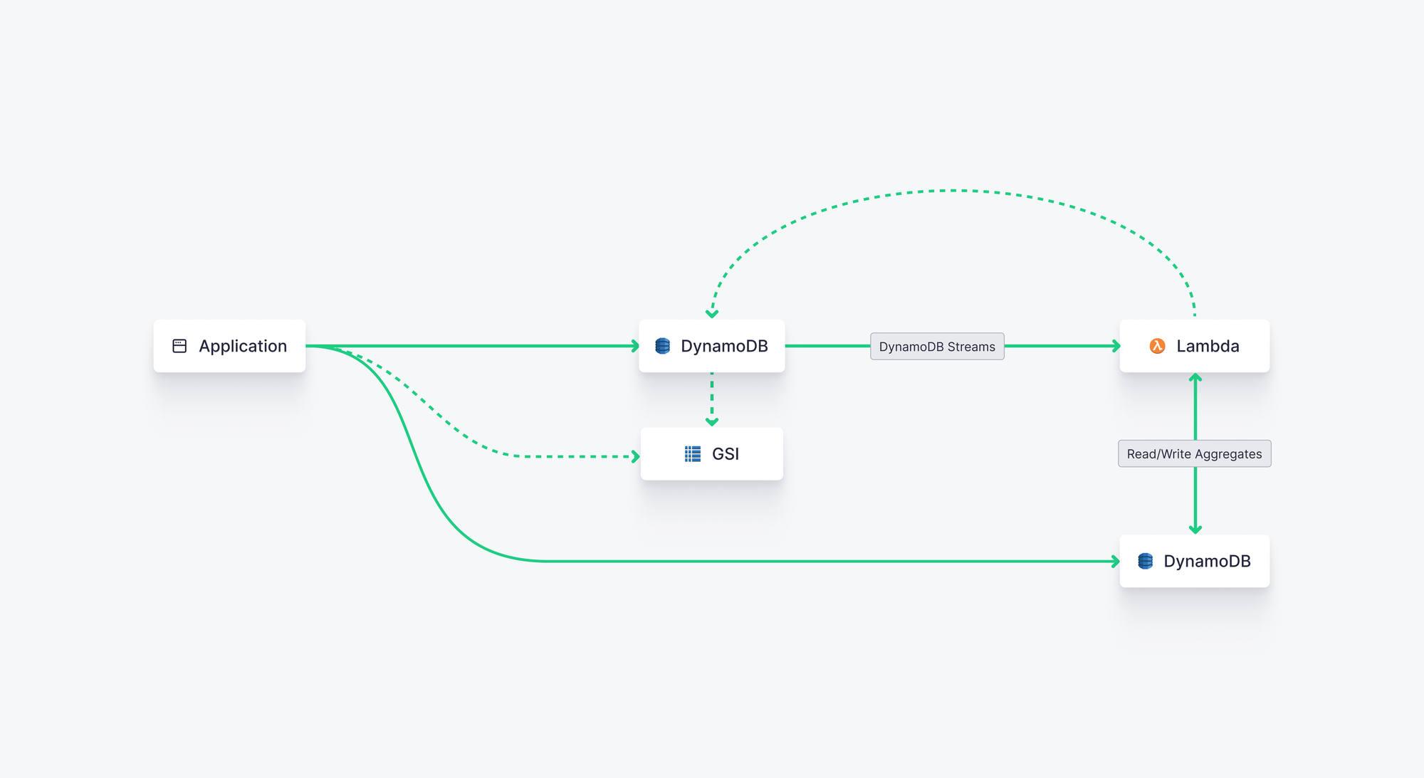
An alternative, especially within the AWS ecosystem, is to use DynamoDB Streams and AWS Lambda for aggregation, a pattern you might be familiar with.

2. The "Batch" Layer (Reconciliation)
For billing, eventual accuracy must be 100%. Stream processors can sometimes make errors or miss events during deployments or failures. The batch layer acts as the source of truth.

• All raw events from the message queue are also durably stored in cheap object storage (e.g., Amazon S3).
• A periodic batch job (e.g., a daily Apache Spark job) runs, reading the complete and immutable raw event log from S3 for the previous day.
• It re-calculates the aggregates with perfect accuracy and overwrites the previous day's data in the database, correcting any discrepancies from the speed layer.

The following video walks through a similar system design, highlighting the benefits of separating workloads and using both stream and batch processing.

This hybrid architecture gives us the best of both worlds: fast, near real-time analytics from the speed layer and the guaranteed accuracy required for billing from the batch layer.

5. Supporting Efficient Queries

With our aggregated_token_usage table in place, complex queries become simple, fast, and efficient. Because the data is partitioned by time and indexed on our key dimensions, the database can quickly isolate the relevant data blocks without scanning the entire dataset.

For example, to get the total cost for a specific user in the current month:

SELECT
    SUM(total_cost_usd) AS monthly_cost
FROM
    aggregated_token_usage
WHERE
    user_id = 'auth-user-12345'
    AND time_bucket_hourly >= '2024-10-01T00:00:00Z'
    AND time_bucket_hourly < '2024-11-01T00:00:00Z';

To get a daily breakdown of usage for a specific model:

SELECT
    DATE(time_bucket_hourly) AS usage_date,
    SUM(sum_input_tokens + sum_output_tokens) AS total_tokens
FROM
    aggregated_token_usage
WHERE
    model_id = 'claude-3-5-sonnet-20240620'
GROUP BY
    usage_date
ORDER BY
    usage_date;

These queries are performant because they operate on a much smaller, pre-aggregated dataset rather than the massive raw event log.

Conclusion

Today, we designed a robust and scalable data model for aggregating LLM token usage. We've moved beyond a simple event log to a sophisticated analytical system capable of powering both real-time dashboards and accurate billing reports.

Key Takeaways:

• Raw event logs are unsuitable for analytical queries at scale. Pre-aggregation is necessary for performance and cost-efficiency.
• Time-Series and OLAP databases are purpose-built for this type of workload, offering high write throughput and fast analytical queries.
• A well-designed schema for aggregated data should include dimensions (user_id, model_id, time), measures (token_counts, cost), and a time_bucket.
• A hybrid (stream/batch) architecture provides both near real-time insights (speed layer) and guaranteed accuracy for billing (batch reconciliation layer).
• This aggregated data model allows for efficient querying by user, model, and time, enabling fast, user-facing analytics and reliable internal reporting.

Next Lesson Preview

Now that we have a solid system for tracking usage and cost, the next logical question is: how can we control and reduce those costs? In our next lesson, we will describe technical strategies for reducing token costs, such as prompt engineering and caching.