Recommended resources
The freely available resources this lesson will direct you to.
- Ultimate Guide To Scaling ML Models - Megatron-LM | ZeRO | DeepSpeed | Mixed Precisionwww.youtube.com
- ZeRO & Fastest BERT: Increasing the scale and speed of deep learning training in DeepSpeedwww.youtube.com
- ZeRO: Memory Optimizations Toward Training Trillion ...aiichironakano.github.io
- Everything about Distributed Training and Efficient Finetuningsumanthrh.com
Introduction
Welcome back. In our previous lesson, we established the fundamental memory challenge in large-scale training: the memory cost per GPU for model states (parameters, gradients, and optimizer states) in standard data parallelism. We introduced the Zero Redundancy Optimizer (ZeRO) as a solution that systematically eliminates this memory redundancy by partitioning these states across devices.
This lesson builds directly on that foundation. Our goal is to move from a high-level overview to a precise, quantitative comparison of the three ZeRO stages. You will learn to analyze the specific memory reduction each stage provides and its corresponding impact on communication volume. Understanding these trade-offs is critical for designing efficient training systems and selecting the right optimization strategy for a given model and hardware configuration.
By the end of this lesson, you will be able to compare the different stages of ZeRO and their corresponding reductions in memory consumption, a key skill for optimizing large model training.
A Framework for Comparison
To systematically compare the ZeRO stages, we'll analyze each one through the lens of four key metrics:
- Partitioned States: Which components of the model state are sharded across devices?
- Replicated States: Which components remain duplicated on every device?
- Per-GPU Memory: The resulting memory footprint per device, expressed as a formula.
- Communication Volume: The total amount of data communicated per step, relative to standard data parallelism.
Let's start by defining our baseline. As we established, for a model with parameters using mixed-precision training with the Adam optimizer:
- Baseline (Standard Data Parallelism):
- Partitioned States: None.
- Replicated States: Parameters (), Gradients (), and Optimizer States ().
- Per-GPU Memory: bytes.
- Communication Volume: bytes. This comes from the
AllReduceoperation on the gradients, where each GPU effectively sends and receives the entire gradient tensor.
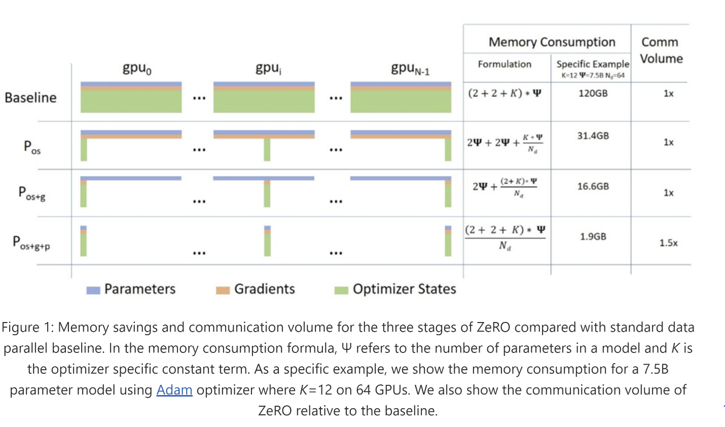
The diagram below, which we saw briefly in the last lesson, provides the essential visual intuition for what follows. It shows how the memory on each GPU (from gpu0 to gpuN-1) is progressively reduced as we move from the baseline to the more aggressive ZeRO stages.
Now, let's dissect each stage using our framework.
ZeRO Stage 1: Optimizer State Partitioning (Pos)
Stage 1 targets the largest single consumer of memory: the optimizer states.
-
Partitioned States: Optimizer States ().
-
Replicated States: FP16 Parameters () and FP16 Gradients ().
-
Per-GPU Memory: The optimizer state memory is sharded across devices. The total per-GPU memory for model states becomes:
As becomes large, the term becomes negligible, and the memory approaches . This represents approximately a 4x reduction from the baseline .
-
Communication Volume: The communication volume remains the same as standard data parallelism (). This is a crucial benefit.
You might wonder how this is possible, since each GPU only updates a partition of the parameters. The process ensures consistency without extra communication:
- Gradients are fully synchronized across all GPUs via a standard
AllReduceoperation. - Each GPU updates its assigned partition of the optimizer states and, consequently, its partition of the master FP32 parameters.
- An
AllGatheroperation is then performed, where each GPU broadcasts its updated parameter partition to all other GPUs.
The key insight is that the standard AllReduce collective can be implemented as a ReduceScatter followed by an AllGather. ZeRO Stage 1 effectively performs the ReduceScatter and AllGather on different data (gradients vs. parameters), but the total volume of data moved remains the same.
[PDF] Memory Optimizations Toward Training Trillion Parameter Models
The original ZeRO paper formally defines Stage 1. Reading this section will solidify your understanding of how it achieves memory savings.
Please read section V-A, 'Pos: Optimizer State Partitioning' (page 5). Focus on the description of the process and the 'Memory Savings' paragraph, which contains the memory formula we just derived.
ZeRO Stage 2: Gradient and Optimizer State Partitioning (Pos+g)
Stage 2 builds on Stage 1 by also partitioning the gradients.
-
Partitioned States: Optimizer States () and Gradients ().
-
Replicated States: FP16 Parameters ().
-
Per-GPU Memory: Now, both gradients and optimizer states are sharded.
For large , the memory approaches , yielding an 8x reduction from the baseline.
-
Communication Volume: Remarkably, the communication volume remains the same as standard data parallelism (). Stage 2 replaces the full
AllReduceon gradients with aReduceScatter. During the backward pass, this operation averages the gradients and distributes to each GPU only the partition it needs for its subsequent parameter update. This avoids storing the full gradient tensor on every device. The communication for the finalAllGatherof updated parameters remains, and the combined volume ofReduceScatter+AllGatheris equivalent to a singleAllReduce.
Everything about Distributed Training and Efficient Finetuning
The following blog post provides an exceptionally clear explanation of the communication pattern in ZeRO Stage 2, clarifying why there's no communication overhead.
Please read the section 'ZeRO Stage 2 / Pos+g (Optimizer State + Gradient Partitioning)'. It details how replacing All-Reduce with Reduce-Scatter for gradients saves memory while keeping communication volume constant.
ZeRO Stage 3: Full State Partitioning (Pos+g+p)
Stage 3 is the most aggressive optimization, partitioning everything.
-
Partitioned States: Optimizer States (), Gradients (), and Parameters ().
-
Replicated States: None (beyond transient buffers).
-
Per-GPU Memory: All model states are now sharded.
This provides a linear memory reduction of -fold. It effectively makes the aggregate memory of all GPUs in the cluster available, enabling the training of models of practically any size.
-
Communication Volume: This is the first stage that increases communication. The volume becomes 1.5x that of standard data parallelism (). The increase comes from the need to gather the full parameters for each layer during the forward and backward passes. The communication flow for each layer is:
AllGatherthe necessary parameters for the current layer's forward computation ( total volume over a full pass).- After the backward pass,
ReduceScatterthe gradients as in Stage 2 ( total volume). - After the local parameter update,
AllGatherthe updated parameters as in S1/S2 is not needed because they are already partitioned. The firstAllGatherof parameters for the next training step handles this. However, the paper's 1.5x figure implies a total of . Let's follow the clearer logic from the blog post:AllGatherfor forward pass () +ReduceScatterfor backward pass () + an additional communication step to sync updated weights, totaling . This modest 50% increase in communication is often a worthwhile price for the massive memory savings.
Everything about Distributed Training and Efficient Finetuning
To understand how the full parameter partitioning works and its impact on communication, let's consult the blog post's clear explanation.
Please read the section 'ZeRO Stage 3 / Pos+g+p (Optimizer State + Gradient + Parameter Partitioning)'. Pay close attention to the breakdown of the communication volume, which explains the source of the 1.5x overhead.
Summary and Quantitative Comparison
Let's consolidate our findings into a summary table.
| Stage | Partitioned States | Per-GPU Memory ( GPUs) | Asymptotic Reduction | Communication Volume |
|---|---|---|---|---|
| Baseline DP | None | 1x | (Baseline) | |
| ZeRO-1 | Optimizer States | 4x | (1x Baseline) | |
| ZeRO-2 | Optimizer States, Gradients | 8x | (1x Baseline) | |
| ZeRO-3 | Parameters, Gradients, Optimizer States | -fold | (1.5x Baseline) |
To see these formulas in action, let's look at the concrete numbers for different model sizes from the original ZeRO paper.
[PDF] Memory Optimizations Toward Training Trillion Parameter Models
The following table from the ZeRO paper provides a powerful quantitative look at the memory savings. It translates our formulas into concrete gigabyte values.
Please examine Table I on page 6. Focus on the row for '64' under the DP degree. Trace the memory consumption for the 7.5B model as you move from Pos to Pos+g and Pos+g+p. Compare this to the baseline value in the first row (Nd=1), which is 120 GB.
As you can see from the table, for a 7.5B parameter model on 64 GPUs:
- Baseline memory is 120 GB.
- ZeRO-1 (
Pos) reduces it to 31.4 GB. - ZeRO-2 (
Pos+g) reduces it further to 16.6 GB. - ZeRO-3 (
Pos+g+p) brings it down to an incredible 1.88 GB.
This clearly demonstrates the power of each successive stage. Finally, let's watch a short summary from one of the creators of ZeRO, which recaps these benefits concisely.
ZeRO & Fastest BERT: Increasing the scale and speed of deep learning training in DeepSpeed
This clip from a Microsoft Research presentation provides a final, authoritative summary of the memory and communication tradeoffs for each ZeRO stage.
Please watch from 35:47 to 37:17. The speaker summarizes the memory reduction factors (4x, 8x, and linear) and confirms the communication overhead profile for each stage.
Conclusion
In this lesson, we conducted a detailed, quantitative comparison of the three stages of the Zero Redundancy Optimizer. By systematically analyzing what each stage partitions, we derived the specific memory savings and communication costs, moving from abstract concepts to concrete formulas and numbers.
Key Takeaways:
- ZeRO-1 partitions optimizer states, offering up to a 4x memory reduction with no communication overhead compared to standard data parallelism.
- ZeRO-2 partitions both optimizer states and gradients, yielding up to an 8x memory reduction, also with no communication overhead.
- ZeRO-3 partitions all model states (parameters, gradients, and optimizer states), achieving a linear -fold memory reduction. This immense memory saving comes at the cost of a modest 1.5x increase in communication volume.
- The choice of ZeRO stage presents a clear design trade-off: Stages 1 and 2 provide significant "free" memory savings, while Stage 3 offers the maximum possible memory reduction at the cost of increased communication and implementation complexity.
Preview of the Next Lesson:
Now that you can precisely compare the ZeRO stages, the next logical step is to understand how these partitioning strategies are realized in practice. In the next lesson, we will explore how memory sharding is implemented in leading frameworks like DeepSpeed (which houses the canonical ZeRO implementation) and PyTorch's native Fully Sharded Data Parallel (FSDP), connecting this theory to the tools used to train today's largest models.