ZeRO: Memory Optimization for Large Models

Introduction

Welcome to the first lesson in our module on memory optimization for large-scale models. In our previous module, we analyzed different architectures for managing distributed training, focusing on the communication patterns of the decentralized AllReduce model versus the centralized Parameter Server. We saw that for tightly-coupled GPU clusters, synchronous AllReduce is the dominant paradigm.

However, even with highly efficient communication, we face another, more fundamental barrier as models scale into the tens and hundreds of billions of parameters: memory. In standard data parallel training, every GPU holds a full copy of the model, its gradients, and the optimizer states. This redundancy consumes enormous amounts of memory, making it impossible to even fit these large models on a single device.

This lesson tackles this memory crisis head-on. We will explore the Zero Redundancy Optimizer (ZeRO), a breakthrough technique developed by Microsoft. You will learn how ZeRO systematically eliminates memory redundancy by partitioning the three key components of a model's state—optimizer states, gradients, and parameters—across a group of data-parallel GPUs. This is the foundational technique that enables the training of today's largest AI models.

The Memory Bottleneck: Where Does It All Go?

A common point of confusion when first encountering large model training is understanding where all the GPU memory goes. For example, a model with 1.5 billion parameters stored in 16-bit floating-point precision (FP16) should only occupy about 3 GB of memory. So why does training it often require a GPU with over 32 GB of memory?

The answer lies in the fact that the model parameters are only one piece of the memory puzzle. During training, we must also store the gradients and, most significantly, the optimizer states.

To understand this, let's analyze the memory requirements for a model with $\Psi$ parameters, trained using the common Adam optimizer with mixed precision.

As the paper details, the memory consumption for the model states breaks down as follows:

• Parameters: In mixed-precision training, we typically work with an FP16 copy of the parameters for faster computation.
  • Memory: $2\Psi$ bytes.
• Gradients: These are computed during the backward pass and are also typically stored in FP16.
  • Memory: $2\Psi$ bytes.
• Optimizer States: This is the largest component. For the Adam optimizer to work reliably in a mixed-precision setting, it maintains several states in full 32-bit precision (FP32):
  1. An FP32 master copy of the parameters for stable updates. Memory: $4\Psi$ bytes.
  2. The first-order momentum (a running average of gradients). Memory: $4\Psi$ bytes.
  3. The second-order momentum, or variance. Memory: $4\Psi$ bytes.
  • Total Optimizer State Memory: $4\Psi +4\Psi +4\Psi =12\Psi$ bytes.

Combining these, the total memory required for the model states is:

In standard data parallelism, this entire $16\Psi$ block of memory is replicated on every GPU. For our 1.5B parameter model ($\Psi =1.5\times 10^9$), this amounts to $16\times 1.5\times 10^9\approx 24$ GB, and this is before accounting for activations and other buffers. This massive redundancy is the problem ZeRO was designed to solve.

The ZeRO Principle: Partitioning to Eliminate Redundancy

The core insight of ZeRO is simple yet powerful: if the model states are replicated on every device in data parallelism, this replication is a redundancy that can be eliminated. Instead of replicating, ZeRO partitions the model states across the available data-parallel devices.

If you have $N_d$ data-parallel devices (GPUs), each device becomes responsible for storing and updating only its $1/N_d$ slice of the model states.

The image below provides a high-level visual of this transformation. The top "Baseline" row shows the standard data parallel approach where all three model states (parameters, gradients, and optimizer states) are replicated on every GPU. The bottom row shows the final stage of ZeRO, where each state is partitioned, dramatically reducing the memory footprint on each individual GPU.

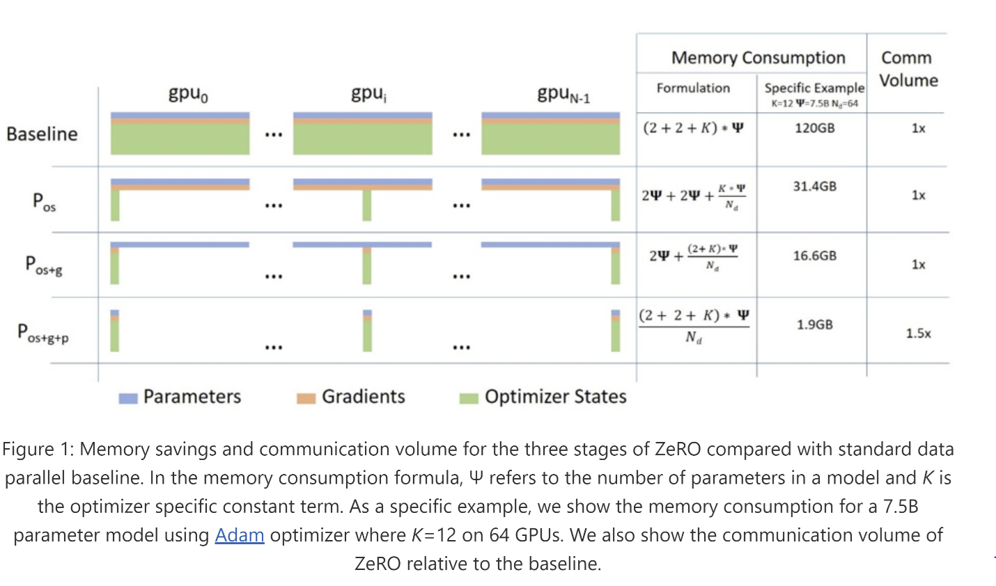
ZeRO implements this partitioning strategy in three incremental stages, allowing a trade-off between memory savings and implementation complexity. Let's examine how each stage works.

The Three Stages of ZeRO Partitioning

Now, let's detail the mechanism behind each stage.

Stage 1: Optimizer State Partitioning (Pos)

• What it partitions: Only the largest portion of the model states—the optimizer states (e.g., the FP32 master parameters, momentum, and variance for Adam). The FP16 parameters and gradients remain replicated on all GPUs.

• How it works:

  1. The forward and backward passes proceed as in standard data parallelism.
  2. An AllReduce operation is performed on the gradients, so every GPU has a complete copy of the averaged gradients.
  3. Each GPU then uses the full gradient tensor to update only its assigned partition of the optimizer states. This is the key step. For example, GPU 0 updates parameters 1 to P/N, GPU 1 updates P/N+1 to 2P/N, and so on.
  4. After updating its local slice of the FP32 master parameters, each GPU has an updated version of a part of the model. An AllGather collective operation is then performed to broadcast these updated parameter partitions to all other GPUs.
  5. At the end of this step, every GPU once again has a complete and updated set of the FP16 parameters, ready for the next forward pass.

• Memory Savings: The optimizer state memory drops from $12\Psi$ to $12\Psi /N_d$. The total memory becomes $4\Psi +12\Psi /N_d$. For a large number of GPUs, this approaches a 4x memory reduction compared to the original $16\Psi$. Critically, the communication volume remains the same as in standard data parallelism.

Stage 2: Gradient and Optimizer State Partitioning (Pos+g)

• What it partitions: Stage 2 builds on Stage 1 by also partitioning the gradients.

• How it works:

  1. During the backward pass, as gradients are computed, they are not collected for a final AllReduce. Instead, a ReduceScatter operation is performed. This collective operation both sums the gradients from all GPUs and scatters them, so that each GPU ends up with only the slice of the final gradients corresponding to the parameter partition it is responsible for.
  2. This avoids the need for each GPU to store the entire gradient tensor, saving $2\Psi$ bytes of memory.
  3. The update step and the final AllGather of parameters proceed as in Stage 1.

• Memory Savings: With both optimizer states and gradients partitioned, the total memory is roughly $2\Psi +(14\Psi )/N_d$. For a large $N_d$, this approaches a 8x memory reduction compared to the original $16\Psi$. Remarkably, this is also achieved with the same communication volume as standard data parallelism, as the ReduceScatter + AllGather combination is equivalent in volume to a single AllReduce.

Stage 3: Parameter, Gradient, and Optimizer State Partitioning (Pos+g+p)

• What it partitions: This is the final and most aggressive stage. It partitions all three model states: parameters, gradients, and optimizer states.

• How it works:

  1. At the beginning of a training step, each GPU holds only a slice of the FP16 parameters.
  2. During the forward and backward passes, as the computation proceeds from one layer to the next, the parameters for the current layer are broadcast from the GPUs that own them to all other GPUs just-in-time for the computation.
  3. Once the layer's computation is finished, the non-local parameters can be freed, minimizing the peak memory usage. This dynamic communication exploits the temporal nature of the training process—you only need the parameters for the layer you are currently computing.
  4. The gradient reduction and parameter updates proceed as in Stage 2, but on a per-partition basis.

• Memory Savings: The memory for all model states is now partitioned. The total memory requirement becomes $(16\Psi )/N_d$. This means the memory consumption per GPU scales linearly with the number of devices, an $N_d$-fold reduction. This enables training models of arbitrary size, provided enough GPUs are available.

• Communication Cost: This stage is the only one that increases the total communication volume, as parameters must be communicated during the forward and backward passes. However, the increase is modest—about 50% more than standard data parallelism—which is often a small price to pay for the enormous memory savings.

Conclusion

In this lesson, we have dissected the ZeRO technique and understood how it addresses the memory wall in large-scale model training. By identifying the massive redundancy in standard data parallel training, ZeRO provides a systematic way to partition model states, enabling a dramatic reduction in per-device memory usage.

Key Takeaways:

• The memory required to train a model is dominated by model states: parameters, gradients, and especially optimizer states, which together can consume $16\times$ the number of parameters in bytes for mixed-precision Adam.
• Standard data parallelism replicates these model states on every GPU, creating a severe memory bottleneck for large models.
• ZeRO (Zero Redundancy Optimizer) eliminates this bottleneck by partitioning the model states across data-parallel devices.
• ZeRO is implemented in three stages, offering a trade-off between memory savings and communication overhead:
  • Stage 1 partitions optimizer states for an up to 4x memory reduction with no communication overhead.
  • Stage 2 adds gradient partitioning for an up to 8x memory reduction, also with no communication overhead.
  • Stage 3 partitions all model states (parameters, gradients, and optimizer states), achieving a full $N_d$-fold memory reduction at the cost of a ~50% increase in communication volume.

Preview of the Next Lesson:

Now that we understand how ZeRO partitions each component of the model state, our next lesson will focus on a more direct and quantitative comparison of these three stages. We will analyze the specific memory savings and communication patterns in greater detail, helping you understand the practical design trade-offs involved in selecting the appropriate ZeRO stage for a given AI system and training workload.