The Kondo Effect: Unveiling Logarithmic Resistivity

Hello! Welcome to the final lesson in our module on Magnetism in Solids.

In our last lesson, we explored the RKKY interaction, which describes how localized magnetic moments in a metal communicate with each other over long distances through the conduction electron sea. This led to an effective, oscillating interaction between pairs of spins. Today, we shift our focus from a pair of impurities to the physics of a single magnetic impurity. We will investigate what happens when this lone impurity interacts with the vast sea of conduction electrons at very low temperatures.

This will lead us to the celebrated Kondo effect. Our goal is to describe this phenomenon and understand its most famous experimental signature: the characteristic logarithmic temperature dependence of resistivity. This effect, a cornerstone of many-body physics, represents a beautiful and subtle problem where simple perturbation theory breaks down, revealing a new, strongly correlated ground state.

1. The Experimental Puzzle: The Resistance Minimum

In an ideal, pure metal, electrical resistivity decreases as temperature is lowered, eventually saturating at a small value determined by static defects. This is because electron-phonon scattering freezes out. However, in the 1930s, experiments on seemingly normal metals like gold revealed a strange anomaly. When doped with a small number of magnetic impurities (like iron), the resistivity would decrease as expected, but then, below a certain temperature, it would turn around and start to increase as the sample was cooled further.

This behavior was completely counter-intuitive. Why would lowering the temperature, which should reduce scattering, lead to higher resistance? The answer, provided by Jun Kondo in 1964, lies in the quantum mechanical nature of the scattering between conduction electrons and the magnetic impurity's spin.

2. The Model: An Impurity Spin in an Electron Sea

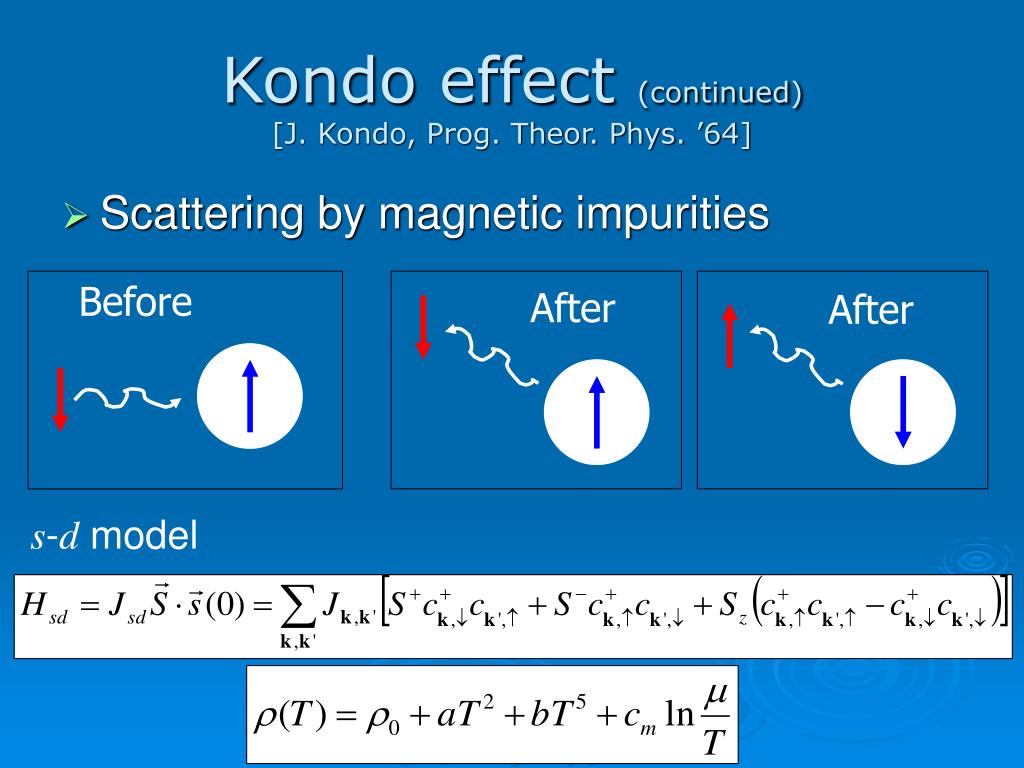
The starting point for understanding this phenomenon is the same local interaction that we used to derive the RKKY interaction. We consider a single magnetic impurity with spin $\mathbf{S}$ placed at the origin of a metal. This spin interacts with the conduction electron spin density, $\mathbf{s}(\mathbf{r})$, only at its location. The Hamiltonian for this interaction is the Kondo Hamiltonian, also known as the s-d model:

$H={\sum }_{\mathbf{k}\sigma }{\epsilon }_{\mathbf{k}}{c}_{\mathbf{k}\sigma }^{†}{c}_{\mathbf{k}\sigma }+J\mathbf{S}\cdot \mathbf{s}(0)$

Here, the first term describes the free conduction electrons, and the second term describes the local exchange interaction. $\mathbf{s}(0)=\frac{1}{2}{\sum }_{\alpha \beta }{\psi }_{\alpha }^{†}(0){\mathbf{\sigma }}_{\alpha \beta }{\psi }_{\beta }(0)$ is the electron spin density operator at the impurity site.

As you may recall from our previous discussions on exchange, the sign of $J$ is crucial. A detailed analysis starting from the more fundamental Anderson model (which describes the hybridization of a localized impurity orbital with the conduction band) shows that this effective interaction is typically antiferromagnetic ($J>0$). This means the conduction electron spins prefer to align anti-parallel to the impurity spin.

3. Kondo's Calculation: The Origin of the Logarithm

Kondo's crucial insight was to calculate the scattering rate of conduction electrons off the magnetic impurity using quantum mechanical perturbation theory beyond the first, simplest approximation. The electrical resistivity due to these impurities, ${\rho }_{mag}$, is proportional to this scattering rate, $1/\tau$.

Let's sketch the key steps of this calculation. The details, which involve applying Fermi's golden rule via the T-matrix formalism, are outlined in the following lecture notes. Your familiarity with diagrammatic approaches from QFT will make the logic here feel quite natural.

As you saw in the reading, the calculation proceeds as follows:

1. First-Order Scattering: Calculating the scattering rate to first order in $J$ (or second order for the rate, $\sim |J{|}^2$) gives a contribution to the resistivity that is independent of temperature. This just adds a constant offset and cannot explain the resistance minimum.

2. Second-Order Scattering: The magic happens when we go to the next order in perturbation theory ($\sim J^3$). In this process, an electron scatters off the impurity, but it does so via an intermediate virtual state. One of these intermediate processes involves the impurity flipping its spin, absorbing an electron-hole pair from the Fermi sea, and then returning to its original state.

   The contribution from this spin-flip process involves an integral over all possible intermediate electron states $q$. This integral has the form:

   $$\sum _{\mathbf{q}}\frac{n_F({\epsilon }_{\mathbf{q}})}{{\epsilon }_{\mathbf{k}}-{\epsilon }_{\mathbf{q}}}\approx {\rho }_0{\int }_{-D}^{0}d\epsilon \frac{1}{{\epsilon }_{\mathbf{k}}-\epsilon }$$

   where $n_F$ is the Fermi-Dirac distribution, ${\rho }_0$ is the density of states at the Fermi level (assumed constant), and $D$ is the conduction band half-width.

3. The Logarithmic Result: For an incoming electron at the Fermi energy (${\epsilon }_{\mathbf{k}}\approx 0$) and at finite temperature $T$, the sharp cutoff of the Fermi function is smeared out over an energy scale of $k_{B}T$. The evaluation of this integral carefully yields a term proportional to $\ln (k_{B}T/D)$.

The final result for the magnetic part of the resistivity is:
${\rho }_{mag}(T)={\rho }_1{J}^2\left(1+2J{\rho }_0\ln \left(\frac{D}{k_{B}T}\right)\right)=c\left(A-B\ln T\right)$
where $c$ is the impurity concentration, and $A$ and $B$ are positive constants. This formula shows that as the temperature $T$ is lowered, the logarithmic term becomes larger and more negative, causing the resistivity to increase.

The total resistivity of the metal is the sum of contributions from electron-phonon scattering (${\rho }_{ph}(T)$) and this magnetic scattering (${\rho }_{mag}(T)$):
${\rho }_{total}(T)={\rho }_{residual}+{\rho }_{ph}(T)+{\rho }_{mag}(T)\approx {\rho }_{res}+\alpha T^5+c(A-B\ln T)$
At high temperatures, the decreasing $\alpha T^5$ term dominates. At low temperatures, the increasing $-B\ln T$ term dominates. The competition between these two opposing trends naturally creates a minimum in the resistivity at a specific temperature, precisely as observed experimentally.

4. The Kondo Problem and the Kondo Temperature

Kondo's perturbative result was a triumph, but it also revealed a deeper problem. Look at the resistivity formula again:
${\rho }_{mag}(T)\propto 1+2J{\rho }_0\ln \left(\frac{D}{k_{B}T}\right)$
What happens as $T\to 0$? The logarithm diverges to $+\infty$, predicting an infinite resistivity! This is unphysical and signals a breakdown of perturbation theory. The interaction, which seems weak at high temperatures, effectively becomes infinitely strong as we approach absolute zero.

This divergence heralds the emergence of a new, non-perturbative energy scale, the Kondo temperature, $T_K$. It is defined as the temperature at which the perturbative correction becomes as large as the leading term:
$1\approx |2J{\rho }_0\ln (D/k_B{T}_K)|$
Solving for $T_K$ gives:
$k_B{T}_K\approx D{e}^{-1/(2J{\rho }_0)}$
This is a remarkable result. $T_K$ depends on the coupling constant $J$ in a non-analytic way (it cannot be expanded in a Taylor series in $J$). This is a hallmark of a strongly correlated, many-body phenomenon.

The physical meaning of $T_K$ is profound:

• For $T\gg T_K$: The impurity acts as a nearly free local magnetic moment. Conduction electrons scatter off it weakly. Kondo's perturbation theory and the $\ln T$ behavior hold in this regime.
• For $T\ll T_K$: The antiferromagnetic coupling $J$ wins. The impurity spin can no longer exist as a free moment. Instead, it captures a cloud of conduction electrons and forms a complex, many-body singlet state with them. The impurity's spin is effectively "screened" or "quenched" by the electron sea. In this low-temperature limit, the system behaves like a non-magnetic scatterer, and the resistivity saturates to a large but finite value.

The transition from the "free moment" regime to the "screened" regime is a smooth crossover centered around $T_K$. This crossover physics cannot be captured by simple perturbation theory and required the development of more powerful theoretical tools, most notably the Renormalization Group (RG), for which Kenneth Wilson won the Nobel Prize in 1982.

The RG approach formalizes the idea of an energy-dependent "running coupling constant" $J(E)$. It shows that as you lower the energy scale $E$, the effective antiferromagnetic coupling grows, leading to the strong-coupling physics below $T_K$.

Conclusion

In this lesson, we have unraveled the mystery of the resistance minimum and entered the fascinating world of the Kondo effect. This phenomenon is a paradigm of many-body physics, demonstrating how a simple-looking interaction can lead to profoundly complex and non-perturbative behavior.

Key Takeaways:

• The Kondo effect describes the screening of a local magnetic impurity by the conduction electrons of a metal at low temperatures.
• Its most famous signature is a contribution to resistivity that behaves as ${\rho }_{mag}\propto -\ln T$, leading to a resistance minimum when combined with phonon scattering.
• The logarithmic dependence arises from second-order spin-flip scattering processes between conduction electrons and the impurity spin.
• The breakdown of this perturbative result at low temperatures defines a new energy scale, the Kondo temperature $T_K$, which separates a high-temperature "free moment" regime from a low-temperature "strong coupling" or "screened moment" regime.
• Below $T_K$, the impurity and surrounding electrons form a non-magnetic, many-body singlet ground state.

Preview of the Next Module

The Kondo problem is a "quantum impurity problem"—the study of a single quantum degree of freedom interacting with a bath. This has proven to be an incredibly fertile ground for developing theoretical techniques. In our next module, "Strongly Correlated Electron Systems," we will scale up from one impurity to a whole lattice of interacting electrons. We will begin by introducing the Hubbard model, the canonical model for studying electron-electron repulsion on a lattice. Many of the concepts we've touched on here—local moments, screening, and the competition between kinetic energy and interaction energy—will reappear in a much richer context.