Budget Constraints and Relative Prices

Introduction

Hello! Welcome back to our study of consumer choice.

In our last lesson, we explored the concept of utility, which is the economist's tool for representing what a consumer wants. We focused on total utility and marginal utility, culminating in the Law of Diminishing Marginal Utility. This principle explains why the satisfaction from consuming more and more of a single good tends to decrease.

However, our wants are unlimited, while our resources are not. This brings us to the other half of the consumer's problem: the constraints they face. Today's lesson focuses on precisely that. We will address the learning outcome: Construct a budget constraint and interpret its slope as the relative price of goods.

We will cover:

• How to define and write the equation for a budget constraint.
• How to graph the budget constraint by finding its intercepts.
• The crucial interpretation of the budget line's slope as both an opportunity cost and the relative price of the goods.

By the end of this lesson, you will have a clear, formal model of what a consumer can afford. This is the second key piece of the puzzle we need to solve for a consumer's optimal choice.

1. What is a Budget Constraint?

A budget constraint represents all the combinations of goods and services that a consumer can afford, given their income and the prices of those goods. It separates the affordable bundles from the unaffordable ones.

Let's start with a short, intuitive video that introduces this idea using a simple example of buying coffee and pizza.

The video makes two essential points:

1. The budget line is the frontier of all possible consumption bundles that exactly exhaust your income.
2. The slope of that line tells you the trade-off between the two goods in the market. The video correctly notes this is the opportunity cost. For example, if a pizza costs $10 and a coffee costs $5, the opportunity cost of one pizza is two coffees.

2. The Algebra of the Budget Line

Your technical background will make the formal representation of the budget constraint quite straightforward. Let's translate the concept into an equation.

If a consumer buys quantities of two goods, which we can call Good X and Good Y, their total spending is the sum of the spending on each good:

Since this spending cannot exceed the consumer's income ($I$), we can write the budget constraint as an inequality:

This inequality represents the budget set—all combinations of X and Y that are affordable.

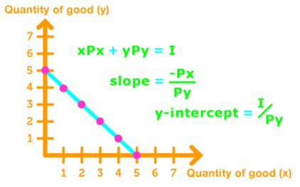
As we assume consumers want to maximize their utility and "more is better" (as discussed last lesson), they will typically spend all their income. This allows us to focus on the frontier of the budget set, which we call the budget line:

3. Deriving and Interpreting the Slope

The most important feature of the budget line is its slope. It contains critical economic information. To see this clearly, we can rearrange the budget line equation into the standard slope-intercept form, $y=mx+b$, where $Y$ is our vertical axis variable.

Starting with the budget line equation:

To isolate $Y$, we first subtract the term for Good X from both sides:

Then, we divide the entire equation by $P_Y$:

In this form, we can see two key components:

• The Y-intercept: $\frac{I}{P_Y}$ is the amount of Good Y you could buy if you spent all your income on Good Y (i.e., if $X=0$).
• The Slope: $-\frac{P_X}{P_Y}$ is the slope of the budget line.

This slope tells us the relative price of the two goods. It's the rate at which the market allows you to trade Good Y for Good X. The negative sign simply indicates that to get more of one good, you must give up some of the other. The magnitude of the slope, $\frac{P_X}{P_Y}$, is the opportunity cost of consuming one more unit of Good X, measured in terms of Good Y.

The following video provides a step-by-step walkthrough of this algebraic derivation and interpretation.

To reinforce this with a textual explanation, the following reading breaks down the same concepts clearly.

4. A Numerical Example

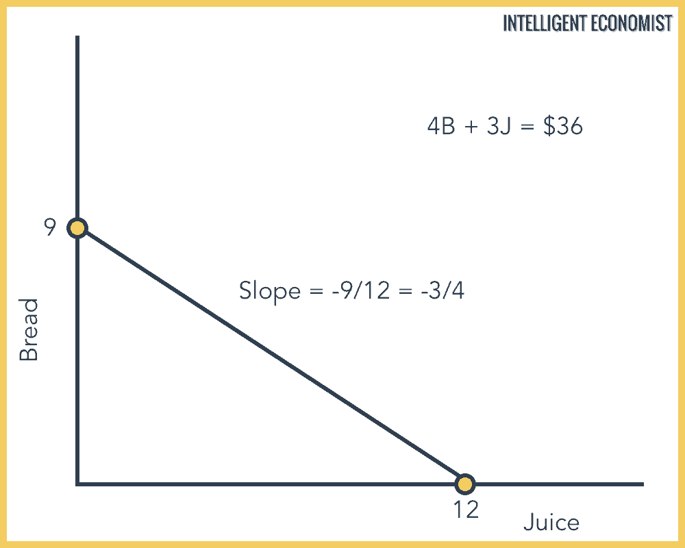
Let's apply these ideas. Suppose you have a budget of $36 to spend on juice ($J$) and bread ($B$). The price of juice is $3 per bottle, and the price of bread is $4 per loaf.

1. The Budget Equation:
   $3J+4B=36$

2. Find the Intercepts:

   • Juice-axis intercept (if $B=0$): If you spend all $36 on juice, you can buy $36/3=12$ bottles. The point is (12, 0) on a graph where juice is on the horizontal axis.
   • Bread-axis intercept (if $J=0$): If you spend all $36 on bread, you can buy $36/4=9$ loaves. The point is (0, 9) on a graph where bread is on the vertical axis.

3. Calculate and Interpret the Slope:
   Let's put Juice on the X-axis and Bread on the Y-axis. The slope is $-\frac{P_J}{P_B}$.
   $\text{Slope}=-\frac{3}{4}$

   • Interpretation: The opportunity cost of one bottle of juice is $\frac{3}{4}$ of a loaf of bread. To get one more bottle of juice, you must give up 0.75 loaves of bread.

Practice Problem

You have a weekly budget of $80 to spend on two goods: burritos and smoothies. The price of a burrito ($X$) is $10, and the price of a smoothie ($Y$) is $5.

1. Write the equation for your budget line.
2. What is the maximum number of burritos you can buy? What is the maximum number of smoothies? (These are your intercepts).
3. Calculate the slope of the budget line.
4. Interpret the slope. What is the opportunity cost of one burrito?

Conclusion

In this lesson, you learned how to model the financial constraints that limit a consumer's choices. This is a crucial step in understanding economic decision-making.

Here are the key takeaways:

• The budget line represents all combinations of two goods that a consumer can purchase by spending their entire income.
• The equation for the budget line is $P_{X}X+P_{Y}Y=I$.
• The slope of the budget line is given by the negative ratio of the prices, $-\frac{P_X}{P_Y}$.
• This slope represents the relative price of the goods and the opportunity cost of consuming one more unit of the good on the horizontal axis.

We have now formally described both what a consumer wants (utility) and what they can afford (the budget constraint). In our next lesson, we will introduce indifference curves, which are a graphical representation of utility. After that, we will be ready to combine the budget constraint and indifference curves to find the single point that represents the consumer's optimal, utility-maximizing choice.